Lecture No. 10
Calculation of local networks (voltage networks) by loss
voltage
Permissible voltage losses in the lines of local networks.
Assumptions underlying the calculation of local networks.
Determination of the greatest voltage loss.
Special cases of calculation of local networks.
Loss of voltage in power lines with a uniformly distributed load.
Permissible voltage losses in the lines of local networks
Local networks include networks with a rated voltage of 6 - 35 kV. The length of local networks significantly exceeds the length of regional networks. The consumption of conductive material and insulating materials significantly exceeds their need for networks of regional significance. This circumstance requires a responsible approach to the design of local networks.
The transmission of electricity from power sources to power receivers is accompanied by a loss of voltage in lines and transformers. Therefore, the voltage at consumers does not remain constant.
Distinguish deviations and fluctuations voltage.
Deviations voltages are due to slow processes of changing loads in individual elements of the network, changing voltage modes on power supplies. As a result of such changes, the voltage at individual points of the network changes in magnitude, deviating from the nominal value.
fluctuations voltages are fast-flowing (at a rate of at least 1% per minute) short-term voltage changes. Occur in case of sharp violations of the normal mode of operation with sudden switching on or off of powerful consumers, short circuits.
Voltage deviations are expressed as a percentage in relation to the rated voltage of the network

Voltage fluctuations are calculated as follows:
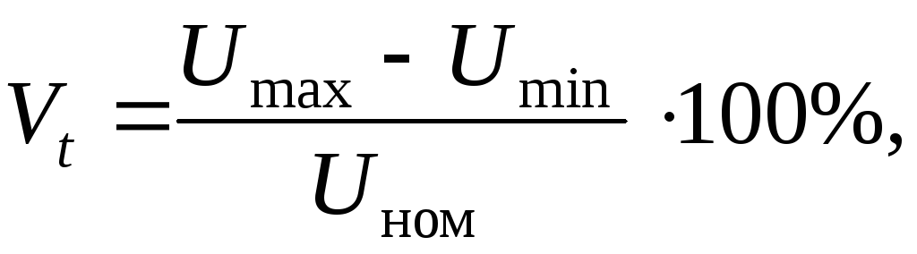
where 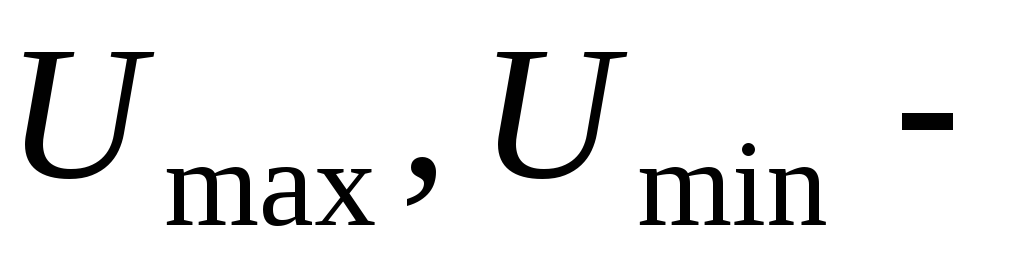 the largest and smallest voltage values at the same point in the network.
To ensure the normal operation of power receivers, it is necessary to maintain a voltage close to the nominal voltage on their tires.
GOST establishes the following permissible deviations in normal operation:
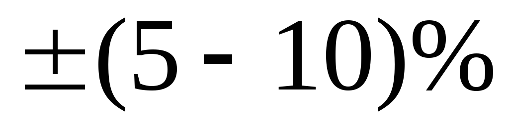
In post-emergency modes, an additional voltage drop of 5% to the specified values is allowed.
To ensure the proper voltage level on the busbars of power receivers, the following measures are used:

With a transformation ratio  the actual voltage on the low voltage busbars will be closer to the nominal:
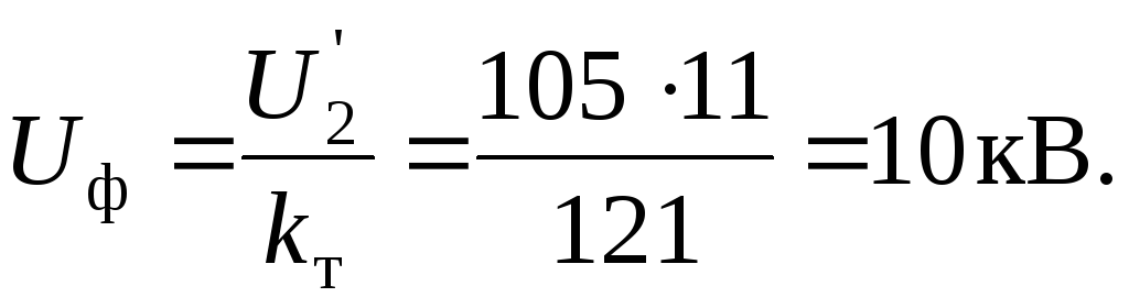
The windings of transformers are equipped with taps that allow you to change the transformation ratio within certain limits. The voltage in the nodes of the circuit located closer to the power source is usually higher than the nominal voltage, and in remote ones it is lower than the nominal voltage. In order to obtain the voltage of the required level on the secondary side of the transformers included in these nodes, it is necessary to select taps in the transformer windings. In nodes with an increased voltage level, transformation ratios are set higher than the nominal value, and in nodes with a reduced voltage level, the transformation ratios of transformers are set below the nominal value.
The network diagram, rated voltage, wire cross-sections are chosen in such a way that the voltage loss does not exceed the allowable value.
The permissible voltage loss is set with a certain degree of accuracy, based on the normalized values of voltage deviations on the buses of power receivers:
for networks with a voltage of 220 - 380 V throughout the entire length from the power source to the last electrical receiver from 5 - 6.5%;
for the supply network with a voltage of 6 - 35 kV - from 6 to 8% in normal mode; from 10 to 12% in the post-accident mode;
for rural networks with a voltage of 6 - 35 kV - up to 10% in normal mode.
These values of permissible voltage loss are selected in such a way that, with proper voltage regulation in the network, the requirements of the Electrical Installation Code for voltage deviations on the buses of power receivers are met.
Assumptions underlying the calculation of local networks
When calculating networks with voltage up to 35 kV inclusive, the following assumptions are made:
the charging power of power lines is not taken into account;
not taken into account inductive reactance cable power lines;
power losses in the steel of transformers are not taken into account. Power losses in the steel of transformers are taken into account only when calculating the losses of active power and electricity in the entire network;
when calculating power flows, power losses are not taken into account, i.e. power at the beginning of the section is equal to the power at the end of the section;
the transverse component of the voltage drop is not taken into account. This means that the voltage shift in phase between the nodes of the circuit is not taken into account;
calculation of voltage losses is carried out according to the rated voltage, and not according to the real voltage in the network nodes.
Determination of the largest voltage loss
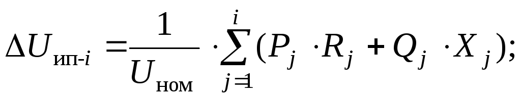
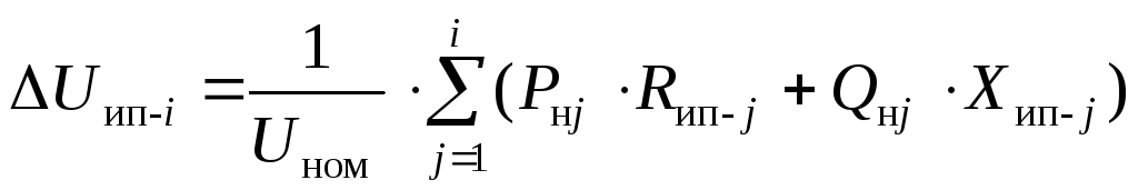
Taking into account the assumptions made when calculating local networks, the voltage in any i-th network node is calculated using a simplified formula:
where  respectively active and reactive power flowing through the section j;
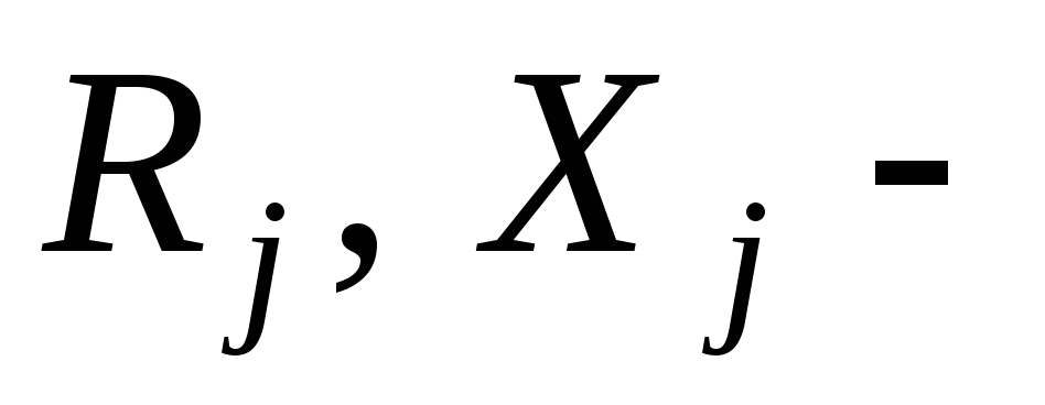 respectively active and inductive resistance of the section j.
Failure to take into account power losses in local networks allows you to calculate voltage losses either by the power of the sections or by the power of the loads.
If the calculation is carried out according to the capacities of the sections, then the active and reactive resistances of the same sections are taken into account. If the calculation is based on the power of the loads, then it is necessary to take into account the total active and reactive resistances from the IP to the load connection node. With regard to fig. 10.2 we have:
![]()
by site capacity
by load power
 .
.
In an unbranched network, the largest voltage loss is the voltage loss from the power supply to the end point of the network.
In a branched network, the largest voltage loss is determined as follows:
the voltage loss from the power supply to each end point is calculated;
among these losses, the largest is selected. Its value should not exceed the allowable voltage loss for this network.
Special cases of calculation of local networks
In practice, there are the following special cases of calculating local networks (the formulas are given for calculating the capacities of the sections):
The power transmission line along the entire length is made with wires of the same section, equally spaced

The power transmission line along the entire length is made with wires of the same section, equally spaced. Loads have the same cosφ
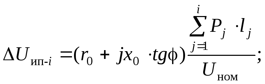
Power lines supplying purely active loads ( Q = 0, cosφ=1), or cable transmission lines with voltage up to 10 kV ( X =0)
Methods for arithmetic calculation of overhead electronic networks with wires from various materials by voltage loss. The allowable voltage loss in the electronic network is determined by the likely allowed voltage deviations for potential users. Therefore, considerable interest has been given to the consideration of a request for a response about voltage deviations.
For any receiver electrical energy specific voltage drops are possible. For example, non-simultaneous power units in standard norms, the allowable deviation of voltage anomalies is ± 5%. This means, therefore, that in a curious incident, if the rated voltage of the provided electric motor is 380 V, from this voltage U "additional = 1.05 Un = 380 x 1.05 = 399 V and U" additional = 0.95 Un = 380 x 0.95 \u003d 361 V should be based on its most likely valid voltage indicators. Of course, that all the buffer voltages included among the designations 361 and 399 V will still satisfy the buying user and compose a certain range, one or another without options can be called the range of desired voltages.
Permissible line voltage loss
Users of electronic energy activity do their workload normally when that voltage is applied to their clamps, based on the mathematical calculation of the manufactured electrical device or apparatus. When transmitting electrical energy through the lines, part of the voltage disappears due to the resistance of the lines themselves and, as a result, at the very end of the strip, i.e., at the buying user, the voltage drops than at the beginning of the line. The drop in voltage from the buying user, when compared with the usual one, is reflected in the operation of the current receiver, even if it is a power or light load.
Because of this, when calculating each power transmission line, voltage differences are not required to exceed with a high probability possible norms, networks generally recognized by the choice of electrical load and calculated for heating, mainly measured by loss, voltage drop.
The voltage drop ΔU is the difference between the voltage at the beginning of the line and at its end. ΔU is usually predetermined in conditionally comparative units of measurement - in relation to the indicated voltage.
When using the opposite voltage regulation, it is possible to increase the likely allowable voltage loss. Unfortunately, its implementation area has limitations. Most of the village users are powered from the busbars of the substations of their area's power system, industrial or municipal. electrical installations. In this case, there may be electricity from substations with a voltage of 35/10 or 110/35 kV.
The voltage loss on the lines of the air rows is calculated by the method for the largest possible load. Since the voltage loss is approximately equal to the increased load at the lowest possible power input, on the lines of the village overhead network, it has highest value 25%.
Permissible voltage loss PUE
PUE is the main document that counts requests for various forms of electrical equipment. The accuracy of the implementation of EMP requests guarantees the error-free and secure operation of electrical installations.
PUE requests are indispensable for all institutions, regardless of formal ownership and organizational and legal forms, as well as for private entrepreneurs and individuals working designers, assembly, adjustment and use of electrical installations.

PUE 7th edition
Voltage levels and control, reactive power compensation:
- Clause 1.2.22. For electric networks, it is necessary to stipulate engineering procedures for guaranteeing the properties of electricity in relation to the request of GOST 13109
- Clause 1.2.23. The voltage adjustment installation must create voltage stabilization on the buses with a voltage of 3-20 kV of substations and power plants, where one or another electrical distribution network is connected, in the range of at least 105%, indicated in the interval of maximum loads and not more than 100%, indicated in the interval of minimum loads of these same networks. The inaccuracy from the mentioned voltage levels must be justified.
- Clause 1.2.24. The alternative and positioning of reactive power compensation devices in power networks is made from the hopelessness of supplying the required network bandwidth in normal and after emergency procedures while maintaining the required voltage levels and endurance reserves.
In distribution networks of 0.4 kV, there is a problem associated with significant voltage imbalances in phases: on loaded phases, the voltage drops to 200 ... 208 V, and on less loaded ones, due to the zero shift, it can increase to 240 V or more. overvoltage may lead to failure electrical appliances and consumer equipment. Voltage asymmetry occurs due to different voltage drops in the line wires during phase current imbalances caused by uneven distribution of single-phase loads. In this case, a current equal to the geometric sum of the phase currents appears in the neutral wire of the four-wire line. In some cases (for example, when the load of one or two phases is disconnected), a current equal to the phase current of the load may flow through the neutral wire. This leads to additional losses in power transmission lines (power lines) 0.4 kV, distribution transformers 10/0.4 kV and, accordingly, in high-voltage networks.
This situation is typical for many rural areas and can occur in residential areas. apartment buildings, where it is practically impossible to evenly distribute the load over the supply phases, as a result of which sufficiently large currents appear in the neutral wire, which leads to additional losses in the conductors of the group and supply lines and makes it necessary to increase the cross section of the neutral working wire to the level of the phase ones.
Voltage imbalances greatly affect the operation of the equipment [L.1]. So a small voltage asymmetry (for example, up to 2%) at the terminals induction motor leads to a significant increase in power losses (up to 33% in the stator and 12% in the rotor), which in turn causes additional heating of the windings and reduces the life of their insulation (by 10.8%), and with distortions of 5%, the total losses increase by 1.5 times and, accordingly, the consumed current increases. Moreover, additional losses due to voltage asymmetry do not depend on the engine load.
With an increase in the voltage on incandescent lamps up to 5%, the luminous flux increases by 20%, and the service life is halved.
On the transformer substations 10 / 0.4 kV, as a rule, transformers with a U / U n connection diagram are installed. It is possible to reduce losses and balance the voltage in a 10 kV power transmission line by applying Y / Zjj or A / Zjj, or (produced by UP METZ named after V.I. Kozlov), but such a replacement is associated with large financial costs and does not compensate for additional losses in the 0.4 kV transmission line.
To compensate for voltage imbalance, it is advisable to redistribute the load currents over the phases, aligning their values.
The need to limit the current of the neutral wire is also caused by the fact that in distribution networks of 0.4 kV, made with a cable, the cross section of the neutral wire is usually taken one step less than the cross section of the phase wire.
In order to reduce power losses in 0.4 kV networks by redistributing currents by phases, limiting the current in the neutral wire and reducing voltage distortions, it is proposed to use a three-phase balancing autotransformer, installing it at the end of the power transmission line, at the load nodes. At the same time, if a short circuit of one of the phases to the neutral wire occurs on the 0.4 kV line to the load node (which unfortunately often happens on overhead power lines in rural areas), consumers downstream of the installed autotransformer will be protected from large overvoltages.
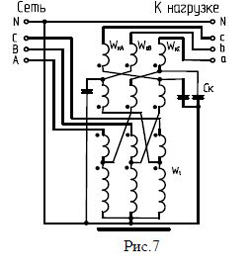
A three-phase, dry, balancing autotransformer (abbreviated as ATS-C) contains a three-rod magnetic circuit, the primary windings W 1 are placed on all three rods, connected in a star with a neutral and connected to the mains voltage, the compensation winding W K is made in the form of an open triangle (some authors call open [L.3]) and connected in series with the load.
The main electrical circuits of the autotransformer are shown in Fig.1...4.
Figure 1 shows circuit diagram an autotransformer with a compensation winding, when the sections of this winding, made on each phase, are connected in a classic open triangle and connected to the network neutral and to the load.
Figure 2 shows the electrical circuit of an autotransformer with a compensation winding made in the form of coils of conductor material lying on top of the windings of all three phases of the autotransformer, forming an open triangle. The use of this scheme, in comparison with the previous one, allows not only to reduce the consumption winding wire additional winding, but also the overall power of the autotransformer by freeing the window of the magnetic circuit and reducing the center distance between the primary windings.
These diagrams are applicable in cases where the neutral conductor of the load does not have a hard connection to earth and in all cases in a five-wire system with PE and N conductors.
Figure 3 shows the electrical circuit of an autotransformer with compensation windings made in the form of phase windings connected in open triangles, connected in accordance with the phase windings of the autotransformer.
Structurally, the circuit shown in Fig. 4 can be performed similarly to the circuit in Fig. 2, i.e. phase compensation windings are made over the windings of all three phases of the autotransformer and are included in the break of the phase wires of the network from the load side.

These schemes can be used, including when the load neutral is solidly grounded, i.e. when it is not possible to include the compensating winding of the autotransformer in the neutral wire break between the load and the network, or when the load neutral wire must be “hard” grounded for safety reasons.
With the asymmetry of the load currents and, accordingly, the currents in the compensation windings, the magnetic fluxes created by these windings in the magnetic circuit of the autotransformer will geometrically add up. In the cores of the magnetic core, zero-sequence flows directed in one direction in all phases of the autotransformer will appear. These magnetic fluxes create emf. zero sequence and, accordingly, currents I 01 in primary winding proportional to the transformation ratio to tr (inversely proportional to the ratio of the number of turns W1 / Wk).
Winding connection W K is chosen in such a way that the phase currents of the autotransformer are vector subtracted from phase current the lines of the most loaded phase and were added to the currents of the less loaded phases. Such a redistribution leads to a more symmetrical distribution of currents by phases in power transmission lines, equalization of voltage drops in the line wires and, consequently, to balancing the voltage at the load, as well as to a decrease in the neutral wire current and losses in the power line and power distribution transformers, providing savings electricity.
The maximum compensation of the current in the neutral wire is performed when the ampere turns (magnetomotive force) of the working I 01 -W 1 and compensation I 02 -W K windings are equal, i.e. at I 01 -W 1 =3I 02 -W K , or W K =W 1 /3. In this case, the overall power of the autotransformer P at, depending on the connection scheme of the compensating windings, can be 3 times less than the power consumption of the load R n.
To limit the current of the neutral wire to the level permissible for power transmission lines, the number of turns of the compensation winding can be correspondingly reduced: for example, to limit the current of the neutral wire at the level of 1/3 of the phase, 2/3 of its value must be compensated, therefore, W K \u003d W 1 / 4.5. In this case, the overall power of the autotransformer can be 4.5 times less than the power consumption of the load.
Distortions of phase currents lead to additional losses in the 0.4 kV power transmission line and further along the entire electricity transmission chain. Consider this on the example of a conditional power line 300 m long, made with an aluminum cable with a cross section of (3x25 + 1x16) mm (phase wire resistance 0.34 Ohm, neutral wire 0.54 Ohm) with an active load in phases 40, 30 and 10A. The current in the neutral wire, equal to the vector sum of the phase currents, will be (see the vector diagram in Fig. 5) 26.5 A. Losses in the line, as in any conductor, depend on the resistance of the line and the square of the current passing through this line (I 2-Z^). Losses in the phase wires, respectively, will be -40 2 -0.34 \u003d 544 W, 30 2 -0.34 \u003d 3 06 W, 10 2 -0.34 \u003d 34 W, in the neutral wire -26.5 -0, 54=379 W, total losses in the line - 1263 W.

The use of ATS-C will redistribute the currents in the line. With a transformation ratio of 1/3, one third of the neutral wire current is vectorially subtracted from the loaded phase currents and added to the current of the less loaded phase. Currents, respectively, will become
Equal to 33.8, 29.6 and 18.6 A, while the neutral wire current (taking into account some asymmetry of the autotransformer magnetic system) can be up to 10% of the average phase current, i.e. 2.7 A.
With such a redistribution of currents, the total losses in the line will be (33.82 + 29.62 + 18.62) 0.34 + 2.72 0.54 = 805W.
Thus, the installation of the ATS-S autotransformer makes it possible to reduce losses in the 0.4 kV power transmission line by 36%.
It is obvious that a decrease in the voltage drop in the line wires is proportional to the change in current in phases, significantly equalizes the voltage in the load node, primarily due to the “zero” shift.
Increasing the transformation ratio above 1/3 for three-phase loads is not advisable and, despite a more uniform redistribution of currents over phases, leads to an increase in losses in power lines due to a more significant increase in the current of the neutral wire, and will also require high costs for materials.
The relative value of the power of the ATS-S autotransformer will be - S * at = k·Sn, where: Sn - load power; k is the coefficient depending on the autotransformer circuit and the transformation ratio (ktr), presented in Table 1.
Table 1 coefficient valuesto
| Scheme, fig. | 1 | 2 | 3 | 4 |
| ktr = 1/3 | 0,58 | 0,33 | 0,90 | 0,55 |
| ktr \u003d 1 / 4.5 | 0,38 | 0,22 | 0,66 | 0,33 |
If the maximum current flowing in the load neutral wire is guaranteed to be known, then the overall power of the autotransformer according to the diagram in Fig. 1 can be calculated based on this current - B at = 1 02 -u l / l / 3, and according to the diagram in Fig. 2 - B at \u003d 1 02 -i l / 3 and for the above example of a three-phase unbalanced load will be, respectively, 8.3 and 4.8 kV-A.
The most effective is the installation of an autotransformer directly at the consumer, at the branching point of a three-phase line into single-phase ones, for example, at the input of a summer cottage, where it is almost impossible to equalize the load across the phases. In residential multi-apartment buildings, the installation of ATS-S on the branches to each riser supplying apartments in residential buildings makes it possible to balance the voltage and reduce losses in three-phase group and supply lines of the distribution network. In small industrial enterprises, it can be used to power single-phase high power loads: welding transformers, rectifiers, water heaters, etc.
Currently, static converters (rectifiers, thyristor regulators, high-frequency converters), gas-discharge lighting devices with electromagnetic and electronic ballasts, electric motors alternating current variable speed, etc. These devices, as well as welding transformers, special medical and other devices, can generate higher current harmonics in the power supply system. For example, single-phase rectifiers can generate all odd harmonics, and three-phase ones can generate all non-multiples of three, which is shown in Fig. 6 [L.2].
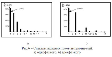
Current harmonics generated by non-linear loads can be serious problems for power supply systems. Harmonic components are currents with frequencies that are multiples of the fundamental frequency of the power supply. The higher harmonics of the current, superimposed on the fundamental harmonic, lead to distortion of the current waveform. In turn, current distortion affects the voltage waveform in the power supply system, causing unacceptable effects on system loads. An increase in the total effective current value in the presence of higher harmonic components in the system can lead to overheating of all distributed network equipment. With non-sinusoidal currents, losses in transformers increase, mainly due to eddy current losses, which requires an increase in their installed power. As a rule, to limit harmonics in these cases, high-frequency filters are installed, consisting of network reactors and capacitors.
The advantages of ATS-S include the fact that they have the ability to filter higher harmonic currents that are multiples of three (i.e. 3, 9, 15, etc.), limiting their flow both from the network to the load, and vice versa. This improves the quality of the network and reduces voltage fluctuations.
As already mentioned above, electromagnetic ballast ballasts (ballasts) of gas discharge lamps generate higher harmonics. So, in the currents of HPS sodium lamps, widely used for the purposes street lighting, the third harmonic is prevailing and, depending on the lamp power and the type of control gear, is up to 5% or more (according to [L.4], the third harmonic is allowed up to 17.5%). The third harmonic currents are in phase and add up arithmetically in the neutral wire three-phase network, creating tangible additional losses, which forces the cross section of zero working conductors of three-phase supply and group lines to be equal to the phase one.
In this situation, the use of ATS-S makes it possible to reduce the cross section of neutral conductors by at least two times and solve three problems: compensate for losses from the third harmonic, ensure that the lighting system is switched to “night mode” (one or two phases of the distribution network are turned off at night ), redistributing the load on three phases; and enter the energy-saving mode by making taps on the autotransformer to lower the voltage. To solve only the first problem, you can use the minimum power autotransformer, designed for the current of the neutral wire (the total current of the third harmonic).
If necessary, compensate for the 5th, 7th or 11th harmonics, you can use the schemes in Fig. 3 or 4. In this case, the cost of network reactors can be reduced, because. compensation windings, having increased inductive resistance for high-frequency harmonics, can act as a network reactor and, together with capacitors, form a higher harmonic filter. Capacitors are connected between the connection points in open triangles of the compensating winding sections and the neutral wire, and can form one (see Fig. 7), two or three-stage filter for different frequencies. The amount of inductance
sections of the compensating winding can be determined with sufficient reliability from the nominal parameters - the rated current and the transformation ratio. For example, when rated current I n \u003d 25A and transformation ratio ktr \u003d 1/3 section voltage
will be U sec \u003d Uf to tr \u003d 220/3 \u003d 73V, resistance Z sec \u003d U sec / Inom \u003d 73/25 \u003d 2.9 Ohm (neglecting the small active resistance of the winding) we consider inductive, and then the inductance of the section
Lsec \u003d Z sec / w \u003d 2.9 / 314-10 \u003d 9.2 mH. In this case, it is necessary to take into account the non-linear nature of the resistance: with a decrease in the load, the resistance increases.
When ordering an autotransformer, the possibility of connecting capacitors must be specified in the application for manufacturing.
A special case is a balancing autotransformer, purposefully designed to power a single-phase load (see Fig. 8 and 9). For greater symmetry of currents in phases, the transformation ratio can be made greater than 1/3, with some increase in the current of the neutral wire.
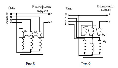
Let's look at this with an example. At the input of the three-phase network, an automatic switch is installed, designed for a long time. admissible current 25 A. It is required to connect a welding transformer with a power of 10 kVA (mains voltage 220 V, welding current 160 A, open circuit voltage 60 V, duty cycle 60%). The current consumed by the welding transformer will be 10-1000/220=45.5 A, and taking into account the PV, the equivalent current will be 45.5-//0.6=35.2 A, which is 1.4 times higher than the allowable one. Of course, you can use a conventional 380/220 V autotransformer, made on the basis of the OSMR-6.3 transformer (with a power of 6.3 kVA), in this case the load will be redistributed only to two phases (line current - 20.3 A), but you can apply a balancing autotransformer (see the diagram in Fig. 9) with a transformation ratio of 1/2, which converts a single-phase load into a three-phase one and equalizes the load in all phases, reducing the current in the network to 17.6 A, while the current is in the neutral, in the absence of other loads it will also be 17.6 A.

In this case, the autotransformer can be made on the basis of the ТСР-6.3 transformer. You can also use a balancing autotransformer with a transformation ratio of 1/3, limiting the current in the working phase to a long-term allowable for circuit breakers- a current of 23.4A, while in the other two phases a current of 11.8A will flow in the absence of current in the neutral wire.
The autotransformer can be made on the basis of the ТСР-2.5 transformer.
The reduction in network losses compared to direct connection is shown in Table 2.
table 2
| Autotransformer | Based on OSMR-6.3 | Balancing ATS-S |
| Transformation ratio | 1/1,73 | 1/3 1/2 |
Given that the welding transformer generates high-frequency harmonics, including multiples of three, preference should be given to a balancing autotransformer.
Tests of autotransformers ATS-S in the laboratory of UE METZ im. IN AND. Kozlov showed positive results and fully confirmed their effectiveness (see Appendix 1 "Test results of the ATS-S-25 autotransformer").
It is planned to develop a series of autotransformers from 25 to 100 kVA both in open version IP00 and in protective casings of IP21 versions for installation under a canopy and IP54 for outdoor installation, including directly on poles of 0.4 kV transmission lines. In autotransformers, if necessary, in order to increase or decrease the voltage, it may be possible to switch the adjusting taps during its installation.
Currently, the plant accepts individual orders for ATS-S autotransformers with a capacity of up to 100 kVA.
Attachment 1
Test results of autotransformer ATS-S-25
On the example of a four-wire transmission line-0.4 kV
| Line length, m | 300 | |||
| Aluminum wire, mm² | phase - | 25 | zero - | 10 |
| Wire resistance, Ohm | phase - | 0,34 | zero - | 0,86 |
| Load resistance (active), Ohm | Phase: A-5.99 | B-5.83 | C-5.59 | |
| Load mode without autotransformer | 3x-f | 2x-f | 1o-f | |
| Line currents load, A | ||||
| phase A | 36,5 | 36,5 | 36,5 | |
| phase B | 37,5 | 37,5 | 0,0 | |
| phase C | 39,0 | 0,0 | 0,0 | |
| in the neutral wire N | 2,2 | 37,0 | 36,5 | |
| phase A | 456 | 456 | 456 | |
| phase B | 481 | 481 | 0 | |
| 520 | 0 | 0 | ||
| in the neutral wire "N" | 4 | 1172 | 1140 | |
| TOTAL | 1461 | 2109 | 1596 | |
| Load mode with autotransformer | 3x-f | 2x-f | 1o-f | |
| Linear currents up to ATS-C, A | ||||
| phase A | 36,0 | 32,5 | 27,3 | |
| phase B | 36,0 | 34,1 | 9,3 | |
| phase C | 39,0 | 9,0 | 8,4 | |
| in the neutral wire "n" | 3,8 | 11,0 | 11 | |
| Power loss in the line, W | ||||
| phase A | 443 | 361 | 255 | |
| phase B | 443 | 398 | 30 | |
| phase C | 520 | 28 | 24 | |
| in the neutral wire N | 12 | 103 | 103 | |
| TOTAL in the line | 1419 | 890 | 412 | |
| taking into account losses in ATS-S | ||||
| phase winding resistance, Ohm | 0,2443 | |||
| compensating winding resistance, Ohm | 0,038 | |||
| Phase winding currents ATS-C, A | ||||
| phase A | 0,4 | 8,1 | 8,9 | |
| phase B | 1,4 | 9,2 | 9,3 | |
| phase C | 1,3 | 8,9 | 8 | |
| Power losses in ATS-S windings, W | ||||
| phase A | 0,04 | 16,03 | 19,35 | |
| phase B | 0,48 | 20,68 | 21,13 | |
| phase C | 0,41 | 19,35 | 15,64 | |
| in the neutral wire N | 0,18 | 52,09 | 50,67 | |
| Idle cold loss ATS-S, W | 50 | |||
| TOTAL in ATS-S | 51,1 | 158,1 | 156,8 | |
| TOTAL | 1470,1 | 1048,2 | 568,8 | |
| Energy saving, W | -8,7 | 1061 | 1027 | |
Consideration of allowable voltage drops in electrical network.
Purpose of the lecture:
Familiarization with the calculations of the load of individual branches of the network.
Permissible voltage drops
With any consumption from the electrical network, there is an occurrence electric current. During its passage, it causes voltage drops on these wires, therefore, the voltage supplied to the power receiver is not equal to the voltage at the power supply terminals, but it is lower. At the same time, different voltage drops are prescribed for individual parts of the electrical wiring.
For the voltage drop from the power supply to the point of consumption, one can proceed from the prescribed voltage deviations (IEC 60 038), which must be between + 6% and - 10% of nominal value(since 2003 these limits should be ). This means that the total voltage drop from the power supply to the point of consumption can be up to 16%.
In the electrical installation of the building itself (i.e. inside the building), according to IEC 60 634-5-52, it is recommended that the voltage drop between the beginning of the installation and the user equipment in use should not exceed 4% of the rated voltage of the installation. This recommendation is somewhat contrary to the requirements of other national standards (eg CSN 33 2130 in the Czech Republic).
It can be assumed that, taking into account the fulfillment of other requirements, when calculating the parameters of the wiring, more drops may occur in a certain segment than indicated above, if the following drops are not exceeded in the wiring from the connection cabinet to the power receiver itself: for lighting leads 4%; at the conclusions for stoves and heaters ( washing machines) 6%; for socket outlets and other terminals 8%.
"Rules for Electrical Installations" (PUE) establish the longest permissible loads(current in amps) for insulated wires. Cables and bare wires, which are shown in the form of a table. These tables are compiled on the basis of theoretical calculations and the results of direct tests of wires and cables for heating.
The maximum allowable loads under heating conditions for wires and cables with aluminum conductors with the same geometric section and the same perimeter with copper conductors should be taken equal to 77% of the loads for the corresponding copper conductors. For power networks, the permissible long-term voltage loss should not exceed 5%, and for lighting networks 2.5% of the nominal.
It can be seen that when summing up all the allowable voltage drops (in the distribution network and in the electrical installation), we can get to the very limit of the performance of some devices and equipment. For example, for relays and contactors, their function is guaranteed from 85% of the rated voltage and above, for electric motors this is from 90% of the rated voltage. Therefore, the above recommendation (voltage drop up to 4%) given in IEC 60 634-5-52 must be followed.
We note that the requirements of national standards do not concern voltage drops on some part of the wiring, but the requirements for how much the voltage can drop in relation to the rated voltage. At the terminals of the transformer, for example, there may be a voltage equal to 110% of the rated voltage, then the voltage drops from them can then be 15%, or 13%. This means that the designer has a certain free space, how to distribute the voltage drops in these cases from the source to the power receiver.
It is necessary to say how the voltage drops are calculated, or how they are summed up. With regard to purely resistive loads, which are electrical thermal electrical equipment, and small cross-sections of wiring, the situation is simple. Voltage drops are the products of currents and wiring resistances that can be in a simple way summarize. In the event that we are talking about electrical equipment, for example, motors, the nature of consumption of which is active and inductive, and the total impedance Z wiring, consisting of a real component (resistance) R and the imaginary component (inductive reactance) X, then these complex quantities are mutually multiplied. The result of this product is again a complex value, which means a complex voltage drop. It describes voltage drops in the real and imaginary coordinate axes. The absolute values of these voltage drops on the individual parts of the wiring from the source to the electrical receiver should therefore not be summed up in the standard way, but should be summed up again only as complex values (i.e. real and imaginary components separately).
Therefore, it should not be surprising that the sums of the absolute values of voltage drops are often not the exact sum of their absolute values on individual wires connected to each other.
Calculation of the load of individual branches of the network
The current loads of individual branches cannot be summarized simply as an arithmetic sum of the absolute values of the currents, but the real and imaginary components must be summed separately. By following these rules, you can determine the load for any network configuration. Similar rules are observed when calculating currents short circuit. And in the event of a short circuit, calculations are performed with the network impedance expressed in complex form.
Influence of load on short circuit current.
The load can have a significant effect on short-circuit currents. Figure 1 shows the simplest load switching schemes. The nature of the loads and their ratios are different (asynchronous and synchronous motors, household load, lighting), the value varies on different days of the year, time of day, for different shifts in the work of enterprises. It is almost impossible to determine the actual value of the load and the increase in its resistance at the time of a short circuit.
Conventionally, it is considered that the load resistance is constant with respect to and the value determined by (1).
In normal mode, the load resistance is determined by the ratio:
![]() , (1)
, (1)
where U is the rated voltage equal to the secondary voltage of the supply transformer;
I n and S n - current and load power.
The load power is taken depending on the number of supply transformers. With one transformer, the load power is assumed to be equal to the power of the transformer. With two identical transformers, the load power is assumed to be 0.65-0.7 of the power of one transformer. At emergency shutdown one of the two transformers, the entire load must be taken by the transformer remaining in operation. In this case, its load will be 130-140% of the rated power.
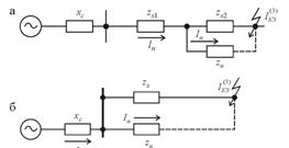
Figure 1 - Current distribution considering the load connected
to the line (a) and to the tires (b)
From figure 1 it can be seen that with a remote short circuit, when the voltage on the buses does not drop to zero, the total current passing through the transformer consists of the current branching into the load and the current at the short circuit location. For the circuit in Figure 1,a, the total short circuit current is determined by the relation:
 , (2)
, (2)
and for the circuit in Figure 1 b - according to the ratio:
 , (3)
, (3)
In fact, the resistances have different x/r ratios, and the currents should be calculated using formulas (2) and (3) in a complex form. But for most networks, the ratio z and L of the load and lines are close, small compared to , and to simplify the calculations, equations (2) and (3) are solved in impedances z. This assumption is all the more justified since the actual load at the moment of short circuit is unknown.
Full current is divided into two parts: part of the current going to the short circuit in the circuit in Figure 1, a, is determined by:
 , (4)
, (4)
and for the circuit in Figure 1, b - according to the formula:
 , (5)
, (5)
It can be seen from expression (5) that at z c = 0, the current to the short circuit is , that is, the load does not affect the value of the short circuit current if it is connected to buses of infinite power.
We advise you to read
 Psychological characteristics of children in adolescence
 Transferring a child to another school - the procedure and necessary documents Whether to transfer a child to another school
, diagnosis, treatment Treatment of urogenital chlamydia") Chlamydia urogenital - description, causes, symptoms (signs), diagnosis, treatment Treatment of urogenital chlamydia
Chlamydia urogenital - description, causes, symptoms (signs), diagnosis, treatment Treatment of urogenital chlamydia The benefits and significance of hydroamino acid threonine for the human body L threonine what