The Gauss method, also called the method of successive elimination of unknowns, consists in the following. Using elementary transformations, the system of linear equations is brought to such a form that its matrix of coefficients turns out to be trapezoidal (same as triangular or stepped) or close to trapezoidal (the direct course of the Gauss method, then - just a direct move). An example of such a system and its solution is shown in the figure above.

In such a system, the last equation contains only one variable and its value can be uniquely found. Then the value of this variable is substituted into the previous equation ( Gaussian reverse , then - just a reverse move), from which the previous variable is found, and so on.

In a trapezoidal (triangular) system, as we see, the third equation no longer contains variables y and x, and the second equation - variable x .

After the matrix of the system has taken a trapezoidal shape, it is no longer difficult to sort out the question of the compatibility of the system, determine the number of solutions, and find the solutions themselves.

Advantages of the method:

1. when solving systems of linear equations with more than three equations and unknowns, the Gauss method is not as cumbersome as the Cramer method, since fewer calculations are required when solving the Gauss method;
2. using the Gauss method, you can solve indefinite systems of linear equations, that is, having a common solution (and we will analyze them in this lesson), and using the Cramer method, you can only state that the system is uncertain;
3. you can solve systems of linear equations in which the number of unknowns is not equal to the number of equations (we will also analyze them in this lesson);
4. the method is based on elementary (school) methods - the method of substitution of unknowns and the method of adding equations, which we touched on in the corresponding article.

In order for everyone to be imbued with the simplicity with which trapezoidal (triangular, step) systems of linear equations are solved, we present the solution of such a system using the reverse stroke. A quick solution to this system was shown in the picture at the beginning of the lesson.

Example 1 Solve a system of linear equations using the reverse move:

Solution. In this trapezoidal system, the variable z is uniquely found from the third equation. We substitute its value into the second equation and get the value of the variable y:

Now we know the values ​​of two variables - z and y. We substitute them into the first equation and get the value of the variable x:

From the previous steps, we write out the solution of the system of equations:

In order to obtain such a trapezoidal system of linear equations, which we solved very simply, it is required to apply a direct move associated with elementary transformations of the system of linear equations. It's also not very difficult.

Elementary transformations of a system of linear equations

Repeating the school method of algebraic addition of the equations of the system, we found out that another equation of the system can be added to one of the equations of the system, and each of the equations can be multiplied by some numbers. As a result, we obtain a system of linear equations equivalent to the given one. In it, one equation already contained only one variable, substituting the value of which into other equations, we come to a solution. Such addition is one of the types of elementary transformation of the system. When using the Gauss method, we can use several types of transformations.

The animation above shows how the system of equations gradually turns into a trapezoidal one. That is, the one that you saw at the very first animation and made sure that it is easy to find the values ​​of all unknowns from it. How to perform such a transformation and, of course, examples, will be discussed further.

When solving systems of linear equations with any number of equations and unknowns in the system of equations and in the expanded matrix of the system can:

1. swap lines (this was mentioned at the very beginning of this article);
2. if as a result of other transformations equal or proportional lines appeared, they can be deleted, except for one;
3. delete "null" rows, where all coefficients are equal to zero;
4. multiply or divide any string by some number;
5. add to any line another line multiplied by some number.

As a result of the transformations, we obtain a system of linear equations equivalent to the given one.

Algorithm and examples of solving by the Gauss method a system of linear equations with a square matrix of the system

Consider first the solution of systems of linear equations in which the number of unknowns is equal to the number of equations. The matrix of such a system is square, that is, the number of rows in it is equal to the number of columns.

Example 2 Solve a system of linear equations using the Gauss method

Solving systems of linear equations using school methods, we multiplied term by term one of the equations by a certain number, so that the coefficients of the first variable in the two equations were opposite numbers. When adding equations, this variable is eliminated. The Gauss method works in a similar way.

To simplify appearance solutions compose the augmented matrix of the system:

In this matrix, the coefficients of the unknowns are located on the left before the vertical bar, and the free members are on the right after the vertical bar.

For the convenience of dividing the coefficients of the variables (to get a division by one) swap the first and second rows of the system matrix. We obtain a system equivalent to the given one, since in the system of linear equations one can rearrange the equations:

With the new first equation eliminate the variable x from the second and all subsequent equations. To do this, add the first row multiplied by (in our case by ) to the second row of the matrix, and the first row multiplied by (in our case by ) to the third row.

This is possible because

If there were more than three equations in our system, then the first line should be added to all subsequent equations, multiplied by the ratio of the corresponding coefficients, taken with a minus sign.

As a result, we obtain a matrix equivalent to the given system of a new system of equations, in which all equations, starting from the second do not contain a variable x :

To simplify the second row of the resulting system, we multiply it by and again get the matrix of the system of equations equivalent to this system:

Now, keeping the first equation of the resulting system unchanged, using the second equation, we eliminate the variable y from all subsequent equations. To do this, add the second row multiplied by (in our case, by ) to the third row of the system matrix.

If there were more than three equations in our system, then the second line should be added to all subsequent equations, multiplied by the ratio of the corresponding coefficients, taken with a minus sign.

As a result, we again obtain the matrix of the system equivalent to the given system of linear equations:

We have obtained a trapezoidal system of linear equations equivalent to the given one:

If the number of equations and variables is greater than in our example, then the process of sequential elimination of variables continues until the system matrix becomes trapezoidal, as in our demo example.

We will find the solution "from the end" - reverse. For this from the last equation we determine z:
.
Substituting this value into the previous equation, find y:

From the first equation find x:

Answer: the solution of this system of equations - .

: in this case, the same answer will be given if the system has a unique solution. If the system has an infinite number of solutions, then so will the answer, and this is the subject of the fifth part of this lesson.

Solve a system of linear equations using the Gauss method yourself, and then look at the solution

Before us is again an example of a consistent and definite system of linear equations, in which the number of equations is equal to the number of unknowns. The difference from our demo example from the algorithm is that there are already four equations and four unknowns.

Example 4 Solve a system of linear equations using the Gauss method:

Now you need to use the second equation to exclude the variable from the subsequent equations. Let's spend preparatory work. To make it more convenient with the ratio of coefficients, you need to get a unit in the second column of the second row. To do this, subtract the third row from the second row, and multiply the resulting second row by -1.

Let us now carry out the actual elimination of the variable from the third and fourth equations. To do this, add the second, multiplied by , to the third line, and the second, multiplied by , to the fourth.

Now, using the third equation, we eliminate the variable from the fourth equation. To do this, to the fourth line, add the third, multiplied by . We get an expanded matrix of a trapezoidal shape.

We have obtained a system of equations, which is equivalent to the given system:

Therefore, the resulting and given systems are consistent and definite. We find the final solution "from the end." From the fourth equation, we can directly express the value of the variable "x fourth":

We substitute this value into the third equation of the system and get

,

,

Finally, value substitution

In the first equation gives

,

where we find "x first":

Answer: This system of equations has a unique solution. .

You can also check the solution of the system on a calculator that solves by Cramer's method: in this case, the same answer will be given if the system has a unique solution.

Solution by the Gauss method of applied problems on the example of a problem for alloys

Systems of linear equations are used to model real objects of the physical world. Let's solve one of these problems - for alloys. Similar tasks - tasks for mixtures, the cost or specific gravity of individual goods in a group of goods, and the like.

Example 5 Three pieces of alloy have a total mass of 150 kg. The first alloy contains 60% copper, the second - 30%, the third - 10%. At the same time, in the second and third alloys taken together, copper is 28.4 kg less than in the first alloy, and in the third alloy, copper is 6.2 kg less than in the second. Find the mass of each piece of alloy.

Solution. We compose a system of linear equations:

Multiplying the second and third equations by 10, we obtain an equivalent system of linear equations:

We compose the extended matrix of the system:

Attention, direct move. By adding (in our case, subtracting) one row, multiplied by a number (we apply it twice), the following transformations occur with the expanded matrix of the system:

The straight run is over. We got an expanded matrix of a trapezoidal shape.

Let's use the reverse. We find a solution from the end. We see that .

From the second equation we find

From the third equation -

You can also check the solution of the system on a calculator that solves by Cramer's method: in this case, the same answer will be given if the system has a unique solution.

The simplicity of the Gauss method is evidenced by the fact that the German mathematician Carl Friedrich Gauss took only 15 minutes to invent it. In addition to the method of his name, from the work of Gauss, the dictum “We should not confuse what seems incredible and unnatural to us with the absolutely impossible” is a kind of brief instruction for making discoveries.

In many applied problems, there may not be a third restriction, that is, a third equation, then it is necessary to solve a system of two equations with three unknowns using the Gauss method, or, conversely, there are fewer unknowns than equations. We now begin to solve such systems of equations.

Using the Gauss method, you can determine whether any system is consistent or inconsistent n linear equations with n variables.

Gauss method and systems of linear equations with an infinite number of solutions

The following example is joint, but indefinite system linear equations, that is, having an infinite number of solutions.

After performing transformations in the expanded matrix of the system (permuting rows, multiplying and dividing rows by a certain number, adding one row to another), rows of the form

If in all equations having the form

The free members are equal to zero, this means that the system is indefinite, that is, it has an infinite number of solutions, and equations of this type are “superfluous” and are excluded from the system.

Example 6

Solution. Let us compose the extended matrix of the system. Then, using the first equation, we eliminate the variable from the subsequent equations. To do this, to the second, third and fourth lines, add the first one, multiplied by , respectively:

Now let's add the second row to the third and fourth.

As a result, we arrive at the system

The last two equations have become equations of the form . These equations are satisfied for any values ​​of the unknowns and can be discarded.

To satisfy the second equation, we can choose arbitrary values ​​for and , then the value for will be determined unambiguously: . From the first equation, the value for is also uniquely found: .

Both the given and the last systems are compatible but indefinite, and the formulas

for arbitrary and give us all solutions of the given system.

Gauss method and systems of linear equations that have no solutions

The following example is an inconsistent system of linear equations, that is, it has no solutions. The answer to such problems is formulated as follows: the system has no solutions.

As already mentioned in connection with the first example, after performing transformations in the expanded matrix of the system, lines of the form

corresponding to an equation of the form

If among them there is at least one equation with a non-zero free term (i.e. ), then this system of equations is inconsistent, that is, it has no solutions, and this completes its solution.

Example 7 Solve the system of linear equations using the Gauss method:

Solution. We compose the extended matrix of the system. Using the first equation, we exclude the variable from the subsequent equations. To do this, add the first multiplied by to the second row, the first multiplied by the third row, and the first multiplied by the fourth row.

Now you need to use the second equation to exclude the variable from the subsequent equations. To obtain integer ratios of the coefficients, we swap the second and third rows of the extended matrix of the system.

To exclude from the third and fourth equations, add the second, multiplied by , to the third row, and the second, multiplied by , to the fourth.

Now, using the third equation, we eliminate the variable from the fourth equation. To do this, to the fourth line, add the third, multiplied by .

The given system is thus equivalent to the following:

The resulting system is inconsistent, since its last equation cannot be satisfied by any values ​​of the unknowns. Therefore, this system has no solutions.

We continue to consider systems of linear equations. This lesson is the third on the topic. If you have a vague idea of ​​what a system of linear equations is in general, you feel like a teapot, then I recommend starting with the basics on the Next page, it is useful to study the lesson.

Gauss method is easy! Why? The famous German mathematician Johann Carl Friedrich Gauss, during his lifetime, received recognition as the greatest mathematician of all time, a genius, and even the nickname "King of Mathematics". And everything ingenious, as you know, is simple! By the way, not only suckers, but also geniuses fall into the money - the portrait of Gauss was flaunted on a bill of 10 Deutschmarks (before the introduction of the euro), and Gauss still mysteriously smiles at the Germans from ordinary postage stamps.

The Gauss method is simple in that it IS ENOUGH THE KNOWLEDGE OF A FIFTH-GRADE STUDENT to master it. Must be able to add and multiply! It is no coincidence that the method of successive elimination of unknowns is often considered by teachers at school mathematical electives. It is a paradox, but the Gauss method causes the greatest difficulties for students. Nothing surprising - it's all about the methodology, and I will try to tell in an accessible form about the algorithm of the method.

First, we systematize the knowledge about systems of linear equations a little. A system of linear equations can:

1) Have a unique solution. 2) Have infinitely many solutions. 3) Have no solutions (be incompatible).

The Gauss method is the most powerful and versatile tool for finding a solution any systems of linear equations. As we remember Cramer's rule and matrix method are unsuitable in cases where the system has infinitely many solutions or is inconsistent. A method of successive elimination of unknowns anyway lead us to the answer! In this lesson, we will again consider the Gauss method for case No. 1 (the only solution to the system), an article is reserved for the situations of points No. 2-3. I note that the method algorithm itself works in the same way in all three cases.

Let's return to the simplest system from the lesson How to solve a system of linear equations? and solve it using the Gaussian method.

The first step is to write extended matrix system: . By what principle the coefficients are recorded, I think everyone can see. The vertical line inside the matrix does not carry any mathematical meaning - it's just a strikethrough for ease of design.

Reference : I recommend to remember terms linear algebra. System Matrix is a matrix composed only of coefficients for unknowns, in this example, the matrix of the system: . Extended System Matrix is the same matrix of the system plus a column of free members, in this case: . Any of the matrices can be called simply a matrix for brevity.

After the extended matrix of the system is written, it is necessary to perform some actions with it, which are also called elementary transformations.

There are the following elementary transformations:

1) Strings matrices can rearrange places. For example, in the matrix under consideration, you can safely rearrange the first and second rows:

2) If there are (or appeared) proportional (as a special case - identical) rows in the matrix, then it follows delete from the matrix, all these rows except one. Consider, for example, the matrix . In this matrix, the last three rows are proportional, so it is enough to leave only one of them: .

3) If a zero row appeared in the matrix during the transformations, then it also follows delete. I will not draw, of course, the zero line is the line in which only zeros.

4) The row of the matrix can be multiply (divide) for any number non-zero. Consider, for example, the matrix . Here it is advisable to divide the first line by -3, and multiply the second line by 2: . This action is very useful, as it simplifies further transformations of the matrix.

5) This transformation causes the most difficulties, but in fact there is nothing complicated either. To the row of the matrix, you can add another string multiplied by a number, different from zero. Consider our matrix from a practical example: . First, I will describe the transformation in great detail. Multiply the first row by -2: , and to the second line we add the first line multiplied by -2: . Now the first line can be divided "back" by -2: . As you can see, the line that is ADDED LI – hasn't changed. Is always the line is changed, TO WHICH ADDED UT.

In practice, of course, they don’t paint in such detail, but write shorter: Once again: to the second line added the first row multiplied by -2. The line is usually multiplied orally or on a draft, while the mental course of calculations is something like this:

“I rewrite the matrix and rewrite the first row: »

First column first. Below I need to get zero. Therefore, I multiply the unit above by -2:, and add the first to the second line: 2 + (-2) = 0. I write the result in the second line: »

“Now the second column. Above -1 times -2: . I add the first to the second line: 1 + 2 = 3. I write the result to the second line: »

“And the third column. Above -5 times -2: . I add the first line to the second line: -7 + 10 = 3. I write the result in the second line: »

Please think carefully about this example and understand the sequential calculation algorithm, if you understand this, then the Gauss method is practically "in your pocket". But, of course, we are still working on this transformation.

Elementary transformations do not change the solution of the system of equations

! ATTENTION: considered manipulations can not use, if you are offered a task where the matrices are given "by themselves". For example, with "classic" matrices in no case should you rearrange something inside the matrices! Let's return to our system. She's practically broken into pieces.

Let us write the augmented matrix of the system and, using elementary transformations, reduce it to stepped view:

(1) The first row was added to the second row, multiplied by -2. And again: why do we multiply the first row by -2? In order to get zero at the bottom, which means getting rid of one variable in the second line.

(2) Divide the second row by 3.

The purpose of elementary transformations – convert the matrix to step form: . In the design of the task, they directly draw out the “ladder” with a simple pencil, and also circle the numbers that are located on the “steps”. The term "stepped view" itself is not entirely theoretical; in the scientific and educational literature, it is often called trapezoidal view or triangular view.

As a result of elementary transformations, we have obtained equivalent original system of equations:

Now the system needs to be "untwisted" in the opposite direction - from the bottom up, this process is called reverse Gauss method.

In the lower equation, we already have the finished result: .

Consider the first equation of the system and substitute the already known value of “y” into it:

Let us consider the most common situation, when the Gaussian method is required to solve a system of three linear equations with three unknowns.

Example 1

Solve the system of equations using the Gauss method:

Let's write the augmented matrix of the system:

Now I will immediately draw the result that we will come to in the course of the solution: 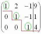And I repeat, our goal is to bring the matrix to a stepped form using elementary transformations. Where to start taking action?

First, look at the top left number: Should almost always be here unit. Generally speaking, -1 (and sometimes other numbers) will also suit, but somehow it has traditionally happened that a unit is usually placed there. How to organize a unit? We look at the first column - we have a finished unit! Transformation one: swap the first and third lines:

Now the first line will remain unchanged until the end of the solution. Now fine.

The unit in the top left is organized. Now you need to get zeros in these places:

Zeros are obtained just with the help of a "difficult" transformation. First, we deal with the second line (2, -1, 3, 13). What needs to be done to get zero in the first position? Need to the second line add the first line multiplied by -2. Mentally or on a draft, we multiply the first line by -2: (-2, -4, 2, -18). And we consistently carry out (again mentally or on a draft) addition, to the second line we add the first line, already multiplied by -2:

The result is written in the second line:

Similarly, we deal with the third line (3, 2, -5, -1). To get zero in the first position, you need to the third line add the first line multiplied by -3. Mentally or on a draft, we multiply the first line by -3: (-3, -6, 3, -27). And to the third line we add the first line multiplied by -3:

The result is written in the third line:

In practice, these actions are usually performed verbally and written down in one step:

No need to count everything at once and at the same time. The order of calculations and "insertion" of results consistent and usually like this: first we rewrite the first line, and puff ourselves quietly - CONSISTENTLY and CAREFULLY:
And I have already considered the mental course of the calculations themselves above.

In this example, this is easy to do, we divide the second line by -5 (since all numbers there are divisible by 5 without a remainder). At the same time, we divide the third line by -2, because the smaller the number, the simpler the solution:

At the final stage of elementary transformations, one more zero must be obtained here:

For this to the third line we add the second line, multiplied by -2:
Try to parse this action yourself - mentally multiply the second line by -2 and carry out the addition.

The last action performed is the hairstyle of the result, divide the third line by 3.

As a result of elementary transformations, an equivalent initial system of linear equations was obtained: Cool.

Now the reverse course of the Gaussian method comes into play. The equations "unwind" from the bottom up.

In the third equation, we already have the finished result:

Let's look at the second equation: . The meaning of "z" is already known, thus:

And finally, the first equation: . "Y" and "Z" are known, the matter is small:

Answer:

As has been repeatedly noted, for any system of equations, it is possible and necessary to check the found solution, fortunately, this is not difficult and fast.

Example 2

This is an example for self-solving, a sample of finishing and an answer at the end of the lesson.

It should be noted that your course of action may not coincide with my course of action, and this is a feature of the Gauss method. But the answers must be the same!

Example 3

Solve a system of linear equations using the Gauss method

We look at the upper left "step". There we should have a unit. The problem is that there are no ones in the first column at all, so nothing can be solved by rearranging the rows. In such cases, the unit must be organized using an elementary transformation. This can usually be done in several ways. I did this: (1) To the first line we add the second line, multiplied by -1. That is, we mentally multiplied the second line by -1 and performed the addition of the first and second lines, while the second line did not change.

Now at the top left "minus one", which suits us perfectly. Who wants to get +1 can perform an additional gesture: multiply the first line by -1 (change its sign).

(2) The first row multiplied by 5 was added to the second row. The first row multiplied by 3 was added to the third row.

(3) The first line was multiplied by -1, in principle, this is for beauty. The sign of the third line was also changed and moved to the second place, thus, on the second “step, we had the desired unit.

(4) The second line multiplied by 2 was added to the third line.

(5) The third row was divided by 3.

A bad sign that indicates a calculation error (less often a typo) is a “bad” bottom line. That is, if we got something like below, and, accordingly, , then with a high degree of probability it can be argued that an error was made in the course of elementary transformations.

We charge the reverse move, in the design of examples, the system itself is often not rewritten, and the equations are “taken directly from the given matrix”. The reverse move, I remind you, works from the bottom up. Yes, here is a gift:

Answer: .

Example 4

Solve a system of linear equations using the Gauss method

This is an example for an independent solution, it is somewhat more complicated. It's okay if someone gets confused. Full solution and design sample at the end of the lesson. Your solution may differ from mine.

In the last part, we consider some features of the Gauss algorithm. The first feature is that sometimes some variables are missing in the equations of the system, for example: How to correctly write the augmented matrix of the system? I already talked about this moment in the lesson. Cramer's rule. Matrix method. In the expanded matrix of the system, we put zeros in place of the missing variables: 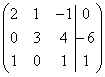By the way, this is a fairly easy example, since there is already one zero in the first column, and there are fewer elementary transformations to perform.

The second feature is this. In all the examples considered, we placed either –1 or +1 on the “steps”. Could there be other numbers? In some cases they can. Consider the system: .

Here on the upper left "step" we have a deuce. But we notice the fact that all the numbers in the first column are divisible by 2 without a remainder - and another two and six. And the deuce at the top left will suit us! At the first step, you need to perform the following transformations: add the first line multiplied by -1 to the second line; to the third line add the first line multiplied by -3. Thus, we will get the desired zeros in the first column.

Or another hypothetical example: . Here, the triple on the second “rung” also suits us, since 12 (the place where we need to get zero) is divisible by 3 without a remainder. It is necessary to carry out the following transformation: to the third line, add the second line, multiplied by -4, as a result of which the zero we need will be obtained.

The Gauss method is universal, but there is one peculiarity. You can confidently learn how to solve systems by other methods (Cramer's method, matrix method) literally from the first time - there is a very rigid algorithm. But in order to feel confident in the Gauss method, you should “fill your hand” and solve at least 5-10 ten systems. Therefore, at first there may be confusion, errors in calculations, and there is nothing unusual or tragic in this.

Rainy autumn weather outside the window .... Therefore, for everyone, a more complex example for an independent solution:

Example 5

Solve a system of 4 linear equations with four unknowns using the Gauss method.

Such a task in practice is not so rare. I think that even a teapot who has studied this page in detail understands the algorithm for solving such a system intuitively. Basically the same - just more action.

The cases when the system has no solutions (inconsistent) or has infinitely many solutions are considered in the lesson. Incompatible systems and systems with a common solution. There you can fix the considered algorithm of the Gauss method.

Wish you success!

Solutions and answers:

Example 2: Solution : Let us write down the extended matrix of the system and, using elementary transformations, bring it to a stepped form.
Performed elementary transformations: (1) The first row was added to the second row, multiplied by -2. The first line was added to the third line, multiplied by -1. Attention! Here it may be tempting to subtract the first from the third line, I strongly do not recommend subtracting - the risk of error greatly increases. We just fold! (2) The sign of the second line was changed (multiplied by -1). The second and third lines have been swapped. note that on the “steps” we are satisfied not only with one, but also with -1, which is even more convenient. (3) To the third line, add the second line, multiplied by 5. (4) The sign of the second line was changed (multiplied by -1). The third line was divided by 14.

Reverse move:

Answer : .

Example 4: Solution : We write the extended matrix of the system and, using elementary transformations, bring it to a step form:

Conversions performed: (1) The second line was added to the first line. Thus, the desired unit is organized on the upper left “step”. (2) The first row multiplied by 7 was added to the second row. The first row multiplied by 6 was added to the third row.

With the second "step" everything is worse , the "candidates" for it are the numbers 17 and 23, and we need either one or -1. Transformations (3) and (4) will be aimed at obtaining the desired unit (3) The second line was added to the third line, multiplied by -1. (4) The third line, multiplied by -3, was added to the second line. The necessary thing on the second step is received . (5) To the third line added the second, multiplied by 6. (6) The second row was multiplied by -1, the third row was divided by -83.

Reverse move:

Answer :

Example 5: Solution : Let us write down the matrix of the system and, using elementary transformations, bring it to a stepwise form:

Conversions performed: (1) The first and second lines have been swapped. (2) The first row was added to the second row, multiplied by -2. The first line was added to the third line, multiplied by -2. The first line was added to the fourth line, multiplied by -3. (3) The second line multiplied by 4 was added to the third line. The second line multiplied by -1 was added to the fourth line. (4) The sign of the second line has been changed. The fourth line was divided by 3 and placed instead of the third line. (5) The third line was added to the fourth line, multiplied by -5.

Reverse move:

Answer :

Ever since the beginning of the 16th-18th centuries, mathematicians began to intensively study the functions, thanks to which so much has changed in our lives. Computer technology without this knowledge simply would not exist. To solve complex problems, linear equations and functions, various concepts, theorems and solution techniques have been created. One of such universal and rational methods and techniques for solving linear equations and their systems was the Gauss method. Matrices, their rank, determinant - everything can be calculated without using complex operations.

What is SLAU

In mathematics, there is the concept of SLAE - a system of linear algebraic equations. What does she represent? This is a set of m equations with the required n unknowns, usually denoted as x, y, z, or x 1 , x 2 ... x n, or other symbols. Solve by Gauss method this system- means to find all the required unknowns. If the system has the same number unknowns and equations, then it is called an n-th order system.

The most popular methods for solving SLAE

AT educational institutions secondary education are studying various techniques for solving such systems. Most often these are simple equations consisting of two unknowns, so any existing method it won't take long to find answers to them. It can be like a substitution method, when another equation is derived from one equation and substituted into the original one. Or term by term subtraction and addition. But the Gauss method is considered the easiest and most universal. It makes it possible to solve equations with any number of unknowns. Why is this technique considered rational? Everything is simple. The matrix method is good because it does not require several times to rewrite unnecessary characters in the form of unknowns, it is enough to do arithmetic operations on the coefficients - and you will get a reliable result.

Where are SLAEs used in practice?

The solution of SLAE are the points of intersection of lines on the graphs of functions. In our high-tech computer age, people who are closely involved in the development of games and other programs need to know how to solve such systems, what they represent and how to check the correctness of the resulting result. Most often, programmers develop special linear algebra calculators, this includes a system of linear equations. The Gauss method allows you to calculate all existing solutions. Other simplified formulas and techniques are also used.

SLAE compatibility criterion

Such a system can only be solved if it is compatible. For clarity, we present the SLAE in the form Ax=b. It has a solution if rang(A) equals rang(A,b). In this case, (A,b) is an extended form matrix that can be obtained from matrix A by rewriting it with free terms. It turns out that solving linear equations using the Gaussian method is quite easy.

Perhaps some notation is not entirely clear, so it is necessary to consider everything with an example. Let's say there is a system: x+y=1; 2x-3y=6. It consists of only two equations in which there are 2 unknowns. The system will have a solution only if the rank of its matrix is ​​equal to the rank of the augmented matrix. What is a rank? This is the number of independent lines of the system. In our case, the rank of the matrix is ​​2. Matrix A will consist of the coefficients located near the unknowns, and the coefficients behind the “=” sign will also fit into the expanded matrix.

Why SLAE can be represented in matrix form

Based on the compatibility criterion according to the proven Kronecker-Capelli theorem, the system of linear algebraic equations can be represented in matrix form. Using the Gaussian cascade method, you can solve the matrix and get the only reliable answer for the entire system. If the rank of an ordinary matrix is ​​equal to the rank of its extended matrix, but less than the number of unknowns, then the system has an infinite number of answers.

Matrix transformations

Before moving on to solving matrices, it is necessary to know what actions can be performed on their elements. There are several elementary transformations:

• By rewriting the system into a matrix form and carrying out its solution, it is possible to multiply all the elements of the series by the same coefficient.
• In order to convert a matrix to canonical form, two parallel rows can be swapped. The canonical form implies that all elements of the matrix that are located along the main diagonal become ones, and the remaining ones become zeros.
• The corresponding elements of the parallel rows of the matrix can be added one to the other.

Jordan-Gauss method

The essence of solving systems of linear homogeneous and inhomogeneous equations by the Gauss method is to gradually eliminate the unknowns. Let's say we have a system of two equations in which there are two unknowns. To find them, you need to check the system for compatibility. The Gaussian equation is solved very simply. It is necessary to write out the coefficients located near each unknown in a matrix form. To solve the system, you need to write out the augmented matrix. If one of the equations contains a smaller number of unknowns, then "0" must be put in place of the missing element. All known transformation methods are applied to the matrix: multiplication, division by a number, adding the corresponding elements of the rows to each other, and others. It turns out that in each row it is necessary to leave one variable with the value "1", the rest should be reduced to zero. For a more accurate understanding, it is necessary to consider the Gauss method with examples.

A simple example of solving a 2x2 system

To begin with, let's take a simple system of algebraic equations, in which there will be 2 unknowns.

Let's rewrite it in an augmented matrix.

To solve this system of linear equations, only two operations are required. We need to bring the matrix to the canonical form so that there are units along the main diagonal. So, translating from the matrix form back into the system, we get the equations: 1x+0y=b1 and 0x+1y=b2, where b1 and b2 are the answers obtained in the process of solving.

1. The first step in solving the augmented matrix will be as follows: the first row must be multiplied by -7 and the corresponding elements added to the second row, respectively, in order to get rid of one unknown in the second equation.
2. Since the solution of equations by the Gauss method implies bringing the matrix to the canonical form, then it is necessary to do the same operations with the first equation and remove the second variable. To do this, we subtract the second line from the first and get the necessary answer - the solution of the SLAE. Or, as shown in the figure, we multiply the second row by a factor of -1 and add the elements of the second row to the first row. This is the same.

As you can see, our system is solved by the Jordan-Gauss method. We rewrite it in the required form: x=-5, y=7.

An example of solving SLAE 3x3

Suppose we have a more complex system of linear equations. The Gauss method makes it possible to calculate the answer even for the most seemingly confusing system. Therefore, in order to delve deeper into the calculation methodology, we can move on to a more complex example with three unknowns.

As in the previous example, we rewrite the system in the form of an expanded matrix and begin to bring it to the canonical form.

To solve this system, you will need to perform much more actions than in the previous example.

1. First you need to make in the first column one single element and the rest zeros. To do this, multiply the first equation by -1 and add the second equation to it. It is important to remember that we rewrite the first line in its original form, and the second - already in a modified form.
2. Next, we remove the same first unknown from the third equation. To do this, we multiply the elements of the first row by -2 and add them to the third row. Now the first and second lines are rewritten in their original form, and the third - already with changes. As you can see from the result, we got the first one at the beginning of the main diagonal of the matrix and the rest are zeros. A few more actions, and the system of equations by the Gauss method will be reliably solved.
3. Now you need to do operations on other elements of the rows. The third and fourth steps can be combined into one. We need to divide the second and third lines by -1 to get rid of the negative ones on the diagonal. We have already brought the third line to the required form.
4. Next, we canonicalize the second line. To do this, we multiply the elements of the third row by -3 and add them to the second line of the matrix. It can be seen from the result that the second line is also reduced to the form we need. It remains to do a few more operations and remove the coefficients of the unknowns from the first row.
5. In order to make 0 from the second element of the row, you need to multiply the third row by -3 and add it to the first row.
6. The next decisive step is to add to the first line necessary elements second row. So we get the canonical form of the matrix, and, accordingly, the answer.

As you can see, the solution of equations by the Gauss method is quite simple.

An example of solving a 4x4 system of equations

Some more complex systems of equations can be solved by the Gaussian method using computer programs. It is necessary to drive coefficients for unknowns into existing empty cells, and the program will calculate the required result step by step, describing each action in detail.

Described below step-by-step instruction solutions to this example.

In the first step, free coefficients and numbers for unknowns are entered into empty cells. Thus, we get the same augmented matrix that we write by hand.

And all the necessary arithmetic operations are performed to bring the extended matrix to the canonical form. It must be understood that the answer to a system of equations is not always integers. Sometimes the solution can be from fractional numbers.

Checking the correctness of the solution

The Jordan-Gauss method provides for checking the correctness of the result. In order to find out whether the coefficients are calculated correctly, you just need to substitute the result into the original system of equations. The left side of the equation must match the right side, which is behind the equals sign. If the answers do not match, then you need to recalculate the system or try to apply another method of solving SLAE known to you, such as substitution or term-by-term subtraction and addition. After all, mathematics is a science that has a huge number of different methods of solving. But remember: the result should always be the same, no matter what solution method you used.

Gauss method: the most common errors in solving SLAE

During the decision linear systems equations, errors such as incorrect transfer of coefficients to matrix form most often occur. There are systems in which some unknowns are missing in one of the equations, then, transferring the data to the expanded matrix, they can be lost. As a result, when solving this system, the result may not correspond to the real one.

Another of the main mistakes can be incorrect writing out the final result. It must be clearly understood that the first coefficient will correspond to the first unknown from the system, the second - to the second, and so on.

The Gauss method describes in detail the solution of linear equations. Thanks to him, it is easy to perform the necessary operations and find the right result. In addition, this is a universal tool for finding a reliable answer to equations of any complexity. Maybe that is why it is so often used in solving SLAE.

Today we deal with the Gauss method for solving systems of linear algebraic equations. You can read about what these systems are in the previous article devoted to solving the same SLAE by the Cramer method. The Gauss method does not require any specific knowledge, only care and consistency are needed. Despite the fact that from the point of view of mathematics, school preparation is enough for its application, mastering this method often causes difficulties for students. In this article, we will try to reduce them to nothing!

Gauss method

M Gauss method is the most universal method for solving SLAE (with the exception of, well, very large systems). Unlike the one discussed earlier, it is suitable not only for systems that have a unique solution, but also for systems that have an infinite number of solutions. There are three options here.

1. The system has a unique solution (the determinant of the main matrix of the system is not equal to zero);
2. The system has an infinite number of solutions;
3. There are no solutions, the system is inconsistent.

So, we have a system (let it have one solution), and we are going to solve it using the Gaussian method. How it works?

The Gaussian method consists of two stages - direct and inverse.

Direct Gauss method

First, we write the augmented matrix of the system. To do this, we add a column of free members to the main matrix.

The whole essence of the Gaussian method is to reduce this matrix to a stepped (or, as they say, triangular) form by means of elementary transformations. In this form, there should be only zeros under (or above) the main diagonal of the matrix.

What can be done:

1. You can rearrange the rows of the matrix;
2. If there are identical (or proportional) rows in the matrix, you can delete all but one of them;
3. You can multiply or divide a string by any number (except zero);
4. Zero lines are removed;
5. You can add a string multiplied by a non-zero number to a string.

Reverse Gauss method

After we transform the system in this way, one unknown xn becomes known, and it is possible to find all the remaining unknowns in reverse order, substituting the already known x's into the equations of the system, up to the first.

When the Internet is always at hand, you can solve the system of equations using the Gauss method online . All you have to do is enter the odds into the online calculator. But you must admit, it is much more pleasant to realize that the example was solved not by a computer program, but by your own brain.

An example of solving a system of equations using the Gauss method

And now - an example, so that everything becomes clear and understandable. Let a system of linear equations be given, and it is necessary to solve it by the Gauss method:

First, let's write the augmented matrix:

Now let's take a look at the transformations. Remember that we need to achieve a triangular form of the matrix. Multiply the 1st row by (3). Multiply the 2nd row by (-1). Let's add the 2nd row to the 1st and get:

Then multiply the 3rd row by (-1). Let's add the 3rd line to the 2nd:

Multiply the 1st row by (6). Multiply the 2nd row by (13). Let's add the 2nd line to the 1st:

Voila - the system is brought to the appropriate form. It remains to find the unknowns:

The system in this example has a unique solution. We will consider the solution of systems with an infinite set of solutions in a separate article. Perhaps at first you will not know where to start with matrix transformations, but after appropriate practice you will get your hands on it and will click the Gaussian SLAE like nuts. And if you suddenly come across a SLAU, which turns out to be too tough a nut to crack, contact our authors! you can by leaving an application in the Correspondence. Together we will solve any problem!

Let us consider exact methods for solving the system ; here is the dimension matrix

A method for solving a problem is classified as exact if, under the assumption that there are no roundings, it gives an exact solution to the problem after a finite number of arithmetic and logical operations. If the number of nonzero elements of the matrix of the system is of the order of , then for most of the currently used exact methods for solving such systems, the required number of operations is of the order of . Therefore, for the applicability of exact methods, it is necessary that such an order of the number of operations be acceptable for a given computer; other restrictions are imposed by the volume and structure of computer memory.

The clause about "methods currently in use" has the following meaning. There are methods for solving such systems with a lower number of operations, but they are not actively used due to the strong sensitivity of the result to the computational error.

The most famous of the exact methods for solving systems of linear equations is the Gauss elimination method. Let's consider one of its possible implementations. Assuming that , the first equation of the system

divide by the coefficient , as a result we obtain the equation

Then, from each of the remaining equations, the first equation is subtracted, multiplied by the appropriate coefficient . As a result, these equations are transformed to the form

The first unknown turned out to be excluded from all equations except the first one. Further, under the assumption that , we divide the second equation by the coefficient and exclude the unknown from all equations, starting from the second, and so on. As a result of successive elimination of unknowns, the system of equations is transformed into a system of equations with a triangular matrix

The set of calculations performed, during which the original problem was transformed to the form (2), is called the direct course of the Gauss method.

From the equation of system (2) we determine , from , etc. up to . The totality of such calculations is called the reverse course of the Gauss method.

It is easy to check that the implementation of the forward move of the Gauss method requires arithmetic operations, and the reverse run requires arithmetic operations.

The exception occurs as a result of the following operations: 1) dividing the equation by , 2) subtracting the equation obtained after such division, multiplied by , from equations with numbers k . The first operation is equivalent to multiplying the system of equations on the left by the diagonal matrix

the second operation is equivalent to multiplication on the left by the matrix

Thus, system (2) obtained as a result of these transformations can be written as

The product of left (right) triangular matrices is a left (right) triangular matrix, so C is a left triangular matrix. From the formula for the elements of the inverse matrix

it follows that the matrix inverse to a left (right) triangular one is a left (right) triangular one. Therefore, the matrix is ​​left triangular.

Let's introduce the notation . According to the construction, everything and the matrix D are right triangular. From here we get the representation of the matrix A as a product of the left and right triangular matrices:

Equality, together with the condition , forms a system of equations with respect to the elements of the triangular matrices B and : . Since for and for , this system can be written as

(3)

or, which is the same,

Using the condition that all we get a system of recurrence relations for determining the elements and :

Calculations are carried out sequentially for sets . Here and below, in the case when the upper summation limit is less than the lower one, it is assumed that the entire sum is equal to zero.

Thus, instead of successive transformations of the system (1) to the form (2), one can directly calculate the matrices B and using formulas (4). These calculations can only be carried out if all elements are different from zero. Let be matrices of principal minors of the order of matrices A, B, D. According to (3) . Because , then . Consequently,

So, in order to carry out calculations according to formulas (4), it is necessary and sufficient to fulfill the conditions

In some cases, it is known in advance that condition (5) is satisfied. For example, many problems of mathematical physics are reduced to solving systems with a positive definite matrix A. However, in general case this cannot be said in advance. Such a case is also possible: everything, but among the quantities there are very small ones, and when divided by them, large numbers with large absolute errors will be obtained. As a result, the solution will be strongly distorted.

Let's denote . Since and , then the equalities hold. Thus, after decomposing the matrix of the original system into the product of left and right triangular matrices, the solution of the original system is reduced to the sequential solution of two systems with triangular matrices; this would require arithmetic operations.

It is often convenient to combine the sequence of operations for decomposing the matrix A into the product of triangular matrices and for determining the vector d. Equations

systems can be written as

Therefore, the values ​​can be calculated simultaneously with the rest of the values ​​using formulas (4).

When solving practical problems, it often becomes necessary to solve systems of equations with a matrix containing a large number of zero elements.

Typically, these matrices have a so-called band structure. More precisely, the matrix A is called -diagonal or has a band structure, if at . The number is called the width of the tape. It turns out that when solving a system of equations with a tape matrix by the Gauss method, the number of arithmetic operations and the required amount of computer memory can be significantly reduced.

Task 1. Investigate the characteristics of the Gauss method and the method of solving the system using the decomposition of the band matrix A into the product of the left and right triangular matrices. Show that arithmetic operations are required to find the solution (for ). Find the leading member of the number of operations under the condition .

Task 2. Estimate the amount of loaded computer memory in the Gauss method for band matrices.

When calculating without the help of a computer, there is a high probability random errors. To eliminate such errors, sometimes a control system is introduced, consisting of control elements of the equations of the system

When transforming equations, the same operations are performed on the control elements as on the free members of the equations. As a result, the control element of each new equation must be equal to the sum of the coefficients of this equation. A large discrepancy between them indicates errors in the calculations or the instability of the calculation algorithm in relation to the computational error.

For example, in the case of bringing the system of equations to the form using formulas (4), the control element of each of the equations of the system is calculated using the same formulas (4). After calculating all the elements at a fixed control is carried out by checking the equality

The reverse course of the Gauss method is also accompanied by the calculation of the control elements of the system rows.

To avoid the catastrophic influence of the computational error, the Gaussian method is used with the choice of the main element.

Its difference from the scheme of the Gaussian method described above is as follows. Let, in the course of eliminating the unknowns, the system of equations

Let us find such that and re-denote and ; then we will eliminate the unknown from all equations, starting with . Such a redesignation leads to a change in the order of elimination of unknowns and in many cases significantly reduces the sensitivity of the solution to rounding errors in calculations.

Often it is required to solve several systems of equations , with the same matrix A. It is convenient to proceed as follows: by introducing the notation

Let us perform calculations using formulas (4), and calculate the elements at . As a result, p systems of equations with a triangular matrix will be obtained, corresponding to the original problem

We solve these systems each separately. It turns out that the total number of arithmetic operations in solving p systems of equations in this way is .

The technique described above is sometimes used in order to obtain a judgment on the error of the solution, which is a consequence of rounding errors in calculations, without significant additional costs. They are given by the vector z with components having, if possible, the same order and sign as the components of the desired solution; often due to lack of sufficient information they take . The vector is calculated, and along with the original system of equations, the system is solved.

Let and z be actually obtained solutions of these systems. Judgment about the error of the desired solution can be obtained based on the hypothesis: the relative errors in solving by the elimination method of systems with the same matrix and different right-hand sides, which are, respectively, the values ​​and , differ not by a very large number of times.

Another technique for obtaining a judgment about the real value of the error that arises due to rounding off in calculations is to change the scale, which changes the picture of the accumulation of the computational error.

Along with the original system, the system is solved by the same method

For and , which are not integer powers of two, the comparison of the vectors and gives an idea of ​​the magnitude of the computational error. For example, you can take .

The study of many problems leads to the need to solve systems of linear equations with a symmetric positive definite matrix. Such systems arise, for example, when solving differential equations finite element method or finite difference methods. In these cases, the matrix of the system also has a band structure.

The method square root(Cholesky method). Matrix A is represented as

where S is a right triangular matrix, is its conjugate, i.e.

with all being a diagonal matrix with elements equal to or -1. Matrix equality (6) forms a system of equations

Similar equations for are discarded, since the equations corresponding to the pairs and are equivalent. From here we obtain recurrent formulas for determining the elements and :

The matrix S is right triangular, and thus, after obtaining representation (6), the solution of the original system also reduces to the Sequential solution of two systems with triangular matrices. Note that in the case of all and .

Task 3. Estimate the number of arithmetic operations and computer memory load (assuming the amount of memory required to store the matrix A decreases) when solving a system with a real positive definite matrix A by the square root method.

Many software packages for solving boundary value problems of mathematical physics by the finite element method are organized according to the following scheme. After the matrix of system A is formed by rearranging rows and columns (both rows and columns are simultaneously rearranged), the system is converted to the form with the smallest tape width. Next, the square root method is applied. At the same time, in order to reduce the amount of calculations when solving a system with other right-hand sides, the matrix S is memorized.