Solving systems of linear algebraic equations, solution methods, examples. System of equations

Systems of equations received wide application in the economic sector mathematical modeling various processes. For example, when solving problems of management and production planning, logistics routes ( transport task) or equipment placement.

Equation systems are used not only in the field of mathematics, but also in physics, chemistry and biology, when solving problems of finding the population size.

system linear equations name two or more equations with several variables for which it is necessary to find a common solution. Such a sequence of numbers for which all equations become true equalities or prove that the sequence does not exist.

Linear Equation

Equations of the form ax+by=c are called linear. The designations x, y are the unknowns, the value of which must be found, b, a are the coefficients of the variables, c is the free term of the equation.
Solving the equation by plotting its graph will look like a straight line, all points of which are the solution of the polynomial.

Types of systems of linear equations

The simplest are examples of systems of linear equations with two variables X and Y.

F1(x, y) = 0 and F2(x, y) = 0, where F1,2 are functions and (x, y) are function variables.

Solve a system of equations - it means to find such values (x, y) for which the system becomes a true equality, or to establish that there are no suitable values of x and y.

A pair of values (x, y), written as point coordinates, is called a solution to a system of linear equations.

If the systems have one common solution or there is no solution, they are called equivalent.

Homogeneous systems of linear equations are systems whose right side is equal to zero. If the right part after the "equal" sign has a value or is expressed by a function, such a system is not homogeneous.

The number of variables can be much more than two, then we should talk about an example of a system of linear equations with three variables or more.

Faced with systems, schoolchildren assume that the number of equations must necessarily coincide with the number of unknowns, but this is not so. The number of equations in the system does not depend on the variables, there can be an arbitrarily large number of them.

Simple and complex methods for solving systems of equations

There is no general analytical way to solve such systems, all methods are based on numerical solutions. The school course of mathematics describes in detail such methods as permutation, algebraic addition, substitution, as well as the graphical and matrix method, the solution by the Gauss method.

The main task in teaching methods of solving is to teach how to correctly analyze the system and find the optimal solution algorithm for each example. The main thing is not to memorize a system of rules and actions for each method, but to understand the principles of applying a particular method.

The solution of examples of systems of linear equations of the 7th grade of the general education school program is quite simple and is explained in great detail. In any textbook on mathematics, this section is given enough attention. The solution of examples of systems of linear equations by the method of Gauss and Cramer is studied in more detail in the first courses of higher educational institutions.

Solution of systems by the substitution method

The actions of the substitution method are aimed at expressing the value of one variable through the second. The expression is substituted into the remaining equation, then it is reduced to a single variable form. The action is repeated depending on the number of unknowns in the system

Let's give an example of a system of linear equations of the 7th class by the substitution method:

As can be seen from the example, the variable x was expressed through F(X) = 7 + Y. The resulting expression, substituted into the 2nd equation of the system in place of X, helped to obtain one variable Y in the 2nd equation. The solution of this example does not cause difficulties and allows you to get the Y value. Last step this is a test of the received values.

It is not always possible to solve an example of a system of linear equations by substitution. The equations can be complex and the expression of the variable in terms of the second unknown will be too cumbersome for further calculations. When there are more than 3 unknowns in the system, the substitution solution is also impractical.

Solution of an example of a system of linear inhomogeneous equations:

Solution using algebraic addition

When searching for a solution to systems by the addition method, term-by-term addition and multiplication of equations by various numbers are performed. The ultimate goal of mathematical operations is an equation with one variable.

For applications this method it takes practice and observation. It is not easy to solve a system of linear equations using the addition method with the number of variables 3 or more. Algebraic addition is useful when the equations contain fractions and decimal numbers.

Solution action algorithm:

Multiply both sides of the equation by some number. As a result of the arithmetic operation, one of the coefficients of the variable must become equal to 1.
Add the resulting expression term by term and find one of the unknowns.
Substitute the resulting value into the 2nd equation of the system to find the remaining variable.

Solution method by introducing a new variable

A new variable can be introduced if the system needs to find a solution for no more than two equations, the number of unknowns should also be no more than two.

The method is used to simplify one of the equations by introducing a new variable. The new equation is solved with respect to the entered unknown, and the resulting value is used to determine the original variable.

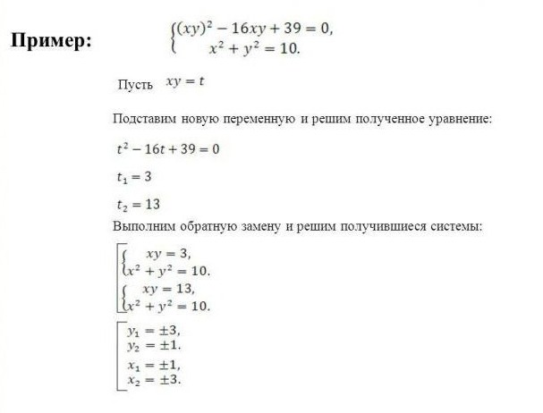
It can be seen from the example that by introducing a new variable t, it was possible to reduce the 1st equation of the system to a standard square trinomial. You can solve a polynomial by finding the discriminant.

It is necessary to find the value of the discriminant using the well-known formula: D = b2 - 4*a*c, where D is the desired discriminant, b, a, c are the multipliers of the polynomial. In the given example, a=1, b=16, c=39, hence D=100. If the discriminant is greater than zero, then there are two solutions: t = -b±√D / 2*a, if the discriminant is less than zero, then there is only one solution: x= -b / 2*a.

The solution for the resulting systems is found by the addition method.

A visual method for solving systems

Suitable for systems with 3 equations. The method consists in plotting graphs of each equation included in the system on the coordinate axis. The coordinates of the points of intersection of the curves and will be common solution systems.

The graphic method has a number of nuances. Consider several examples of solving systems of linear equations in a visual way.

As can be seen from the example, two points were constructed for each line, the values of the variable x were chosen arbitrarily: 0 and 3. Based on the values of x, the values for y were found: 3 and 0. Points with coordinates (0, 3) and (3, 0) were marked on the graph and connected by a line.

The steps must be repeated for the second equation. The point of intersection of the lines is the solution of the system.

In the following example, it is required to find a graphical solution to the system of linear equations: 0.5x-y+2=0 and 0.5x-y-1=0.

As can be seen from the example, the system has no solution, because the graphs are parallel and do not intersect along their entire length.

The systems from Examples 2 and 3 are similar, but when constructed, it becomes obvious that their solutions are different. It should be remembered that it is not always possible to say whether the system has a solution or not, it is always necessary to build a graph.

Matrix and its varieties

Matrices are used to briefly write down a system of linear equations. A matrix is a special type of table filled with numbers. n*m has n - rows and m - columns.

A matrix is square when the number of columns and rows is equal. A matrix-vector is a single-column matrix with an infinitely possible number of rows. A matrix with units along one of the diagonals and other zero elements is called identity.

An inverse matrix is such a matrix, when multiplied by which the original one turns into a unit one, such a matrix exists only for the original square one.

Rules for transforming a system of equations into a matrix

With regard to systems of equations, the coefficients and free members of the equations are written as numbers of the matrix, one equation is one row of the matrix.

A matrix row is called non-zero if at least one element of the row is not equal to zero. Therefore, if in any of the equations the number of variables differs, then it is necessary to enter zero in place of the missing unknown.

The columns of the matrix must strictly correspond to the variables. This means that the coefficients of the variable x can only be written in one column, for example the first, the coefficient of the unknown y - only in the second.

When multiplying a matrix, all matrix elements are successively multiplied by a number.

Options for finding the inverse matrix

The formula for finding the inverse matrix is quite simple: K -1 = 1 / |K|, where K -1 is the inverse matrix and |K| - matrix determinant. |K| must not be equal to zero, then the system has a solution.

The determinant is easily calculated for a two-by-two matrix, it is only necessary to multiply the elements diagonally by each other. For the "three by three" option, there is a formula |K|=a 1 b 2 c 3 + a 1 b 3 c 2 + a 3 b 1 c 2 + a 2 b 3 c 1 + a 2 b 1 c 3 + a 3 b 2 c 1 . You can use the formula, or you can remember that you need to take one element from each row and each column so that the column and row numbers of the elements do not repeat in the product.

Solution of examples of systems of linear equations by the matrix method

The matrix method of finding a solution makes it possible to reduce cumbersome entries when solving systems with a large number of variables and equations.

In the example, a nm are the coefficients of the equations, the matrix is a vector x n are the variables, and b n are the free terms.

Solution of systems by the Gauss method

In higher mathematics, the Gauss method is studied together with the Cramer method, and the process of finding a solution to systems is called the Gauss-Cramer method of solving. These methods are used to find the variables of systems with a large number of linear equations.

The Gaussian method is very similar to substitution and algebraic addition solutions, but is more systematic. In the school course, the Gaussian solution is used for systems of 3 and 4 equations. The purpose of the method is to bring the system to the form of an inverted trapezoid. By algebraic transformations and substitutions, the value of one variable is found in one of the equations of the system. The second equation is an expression with 2 unknowns, and 3 and 4 - with 3 and 4 variables, respectively.

After bringing the system to the described form, the further solution is reduced to the sequential substitution of known variables into the equations of the system.

AT school textbooks for grade 7, an example of a solution by the Gauss method is described as follows:

As can be seen from the example, at step (3) two equations were obtained 3x 3 -2x 4 =11 and 3x 3 +2x 4 =7. The solution of any of the equations will allow you to find out one of the variables x n.

Theorem 5, which is mentioned in the text, states that if one of the equations of the system is replaced by an equivalent one, then the resulting system will also be equivalent to the original one.

The Gauss method is difficult for students to understand high school, but is one of the most interesting ways to develop the ingenuity of children enrolled in the program in-depth study in math and physics classes.

For ease of recording calculations, it is customary to do the following:

Equation coefficients and free terms are written in the form of a matrix, where each row of the matrix corresponds to one of the equations of the system. separates the left side of the equation from the right side. Roman numerals denote the numbers of equations in the system.

First, they write down the matrix with which to work, then all the actions carried out with one of the rows. The resulting matrix is written after the "arrow" sign and continue to perform the necessary algebraic operations until the result is achieved.

As a result, a matrix should be obtained in which one of the diagonals is 1, and all other coefficients are equal to zero, that is, the matrix is reduced to a single form. We must not forget to make calculations with the numbers of both sides of the equation.

This notation is less cumbersome and allows you not to be distracted by listing numerous unknowns.

The free application of any method of solution will require care and a certain amount of experience. Not all methods are applied. Some ways of finding solutions are more preferable in a particular area of human activity, while others exist for the purpose of learning.

Systems of linear equations. Lecture 6

Systems of linear equations.

Basic concepts.

view system

called system - linear equations with unknowns.

Numbers , , are called system coefficients.

Numbers are called free members of the system, – system variables. Matrix

called the main matrix of the system, and the matrix

– expanded matrix system. Matrices - columns

And correspondingly matrices of free members and unknowns of the system. Then, in matrix form, the system of equations can be written as . System solution is called the values of the variables, when substituting which, all the equations of the system turn into true numerical equalities. Any solution of the system can be represented as a matrix-column. Then the matrix equality is true.

The system of equations is called joint if it has at least one solution and incompatible if it has no solution.

To solve a system of linear equations means to find out whether it is compatible and, if it is compatible, to find its general solution.

The system is called homogeneous if all its free terms are equal to zero. A homogeneous system is always compatible because it has a solution

The Kronecker-Kopelli theorem.

The answer to the question of the existence of solutions of linear systems and their uniqueness allows us to obtain the following result, which can be formulated as the following statements about a system of linear equations with unknowns

(1)

Theorem 2. The system of linear equations (1) is consistent if and only if the rank of the main matrix is equal to the rank of the extended one (.

Theorem 3. If the rank of the main matrix of a joint system of linear equations is equal to the number of unknowns, then the system has a unique solution.

Theorem 4. If the rank of the main matrix of a joint system is less than the number of unknowns, then the system has an infinite number of solutions.

Rules for solving systems.

3. Find the expression of the main variables in terms of the free ones and get the general solution of the system.

4. By giving arbitrary values to free variables, all values of the main variables are obtained.

Methods for solving systems of linear equations.

Inverse matrix method.

and , i.e., the system has a unique solution. We write the system in matrix form

where , , .

Multiply both sides of the matrix equation on the left by the matrix

Since , we obtain , from which we obtain equality for finding unknowns

Example 27. Using the inverse matrix method, solve the system of linear equations

Solution. Denote by the main matrix of the system

Let , then we find the solution by the formula .

Let's calculate .

Since , then the system has a unique solution. Find all algebraic additions

, ,

In this way

Let's check

The inverse matrix is found correctly. From here, using the formula , we find the matrix of variables .

Comparing the values of the matrices, we get the answer: .

Cramer's method.

Let a system of linear equations with unknowns be given

and , i.e., the system has a unique solution. We write the solution of the system in matrix form or

Denote

. . . . . . . . . . . . . . ,

Thus, we obtain formulas for finding the values of the unknowns, which are called Cramer's formulas.

Example 28. Solve the following system of linear equations using Cramer's method .

Solution. Find the determinant of the main matrix of the system

Since , then , the system has a unique solution.

Find the remaining determinants for Cramer's formulas

Using Cramer's formulas, we find the values of the variables

Gauss method.

The method consists in sequential exclusion of variables.

Let a system of linear equations with unknowns be given.

The Gaussian solution process consists of two steps:

At the first stage, the extended matrix of the system is reduced to the stepwise form with the help of elementary transformations

where , which corresponds to the system

After that the variables are considered free and in each equation are transferred to right side.

At the second stage, the variable is expressed from the last equation, the resulting value is substituted into the equation. From this equation

variable is expressed. This process continues until the first equation. The result is an expression of the principal variables in terms of the free variables .

Example 29. Solve the following system using the Gaussian method

Solution. Let us write out the extended matrix of the system and reduce it to the step form

Because is greater than the number of unknowns, then the system is compatible and has an infinite number of solutions. Let us write down the system for the step matrix

The determinant of the extended matrix of this system, composed of the first three columns, is not equal to zero, so we consider it to be basic. Variables

Will be basic and the variable will be free. Let's move it in all equations to the left side

From the last equation we express

Substituting this value into the penultimate second equation, we get

where . Substituting the values of the variables and into the first equation, we find . We write the answer in the following form

A system of linear equations is a union of n linear equations, each containing k variables. It is written like this:

Many, when faced with higher algebra for the first time, mistakenly believe that the number of equations must necessarily coincide with the number of variables. In school algebra this is usually the case, but for higher algebra this is, generally speaking, not true.

The solution of a system of equations is a sequence of numbers (k 1 , k 2 , ..., k n ), which is the solution to each equation of the system, i.e. when substituting into this equation instead of variables x 1 , x 2 , ..., x n gives the correct numerical equality.

Accordingly, to solve a system of equations means to find the set of all its solutions or to prove that this set is empty. Since the number of equations and the number of unknowns may not be the same, three cases are possible:

The system is inconsistent, i.e. the set of all solutions is empty. A fairly rare case that is easily detected regardless of which method to solve the system.
The system is consistent and defined, i.e. has exactly one solution. The classic version, well known since school.
The system is consistent and undefined, i.e. has infinitely many solutions. This is the hardest option. It is not enough to state that "the system has an infinite set of solutions" - it is necessary to describe how this set is arranged.

The variable x i is called allowed if it is included in only one equation of the system, and with a coefficient of 1. In other words, in the remaining equations, the coefficient for the variable x i must be equal to zero.

If we select one allowed variable in each equation, we get a set of allowed variables for the entire system of equations. The system itself, written in this form, will also be called allowed. Generally speaking, one and the same initial system can be reduced to different allowed systems, but this does not concern us now. Here are examples of allowed systems:

Both systems are allowed with respect to the variables x 1 , x 3 and x 4 . However, with the same success it can be argued that the second system is allowed with respect to x 1 , x 3 and x 5 . It is enough to rewrite the latest equation in the form x 5 = x 4 .

Now consider more general case. Suppose we have k variables in total, of which r are allowed. Then two cases are possible:

The number of allowed variables r is equal to the total number of variables k : r = k . We get a system of k equations in which r = k allowed variables. Such a system is collaborative and definite, because x 1 \u003d b 1, x 2 \u003d b 2, ..., x k \u003d b k;
The number of allowed variables r is less than the total number of variables k : r< k . Остальные (k − r ) переменных называются свободными - они могут принимать любые значения, из которых легко вычисляются разрешенные переменные.

So, in the above systems, the variables x 2 , x 5 , x 6 (for the first system) and x 2 , x 5 (for the second) are free. The case when there are free variables is better formulated as a theorem:

Please note: this is very important point! Depending on how you write the final system, the same variable can be both allowed and free. Most advanced math tutors recommend writing out variables in lexicographic order, i.e. ascending index. However, you don't have to follow this advice at all.

Theorem. If in a system of n equations the variables x 1 , x 2 , ..., x r are allowed, and x r + 1 , x r + 2 , ..., x k are free, then:

If we set the values of free variables (x r + 1 = t r + 1 , x r + 2 = t r + 2 , ..., x k = t k ), and then find the values x 1 , x 2 , ..., x r , we get one of solutions.

If the values of the free variables in two solutions are the same, then the values of the allowed variables are also the same, i.e. solutions are equal.

What is the meaning of this theorem? To obtain all solutions of the allowed system of equations, it suffices to single out the free variables. Then, assigning to free variables different meanings, we will receive turnkey solutions. That's all - in this way you can get all the solutions of the system. There are no other solutions.

Conclusion: the allowed system of equations is always consistent. If the number of equations in the allowed system is equal to the number of variables, the system will be definite; if less, it will be indefinite.

And everything would be fine, but the question arises: how to get the resolved one from the original system of equations? For this there is

Lesson content

Linear Equations with Two Variables

The student has 200 rubles to have lunch at school. A cake costs 25 rubles, and a cup of coffee costs 10 rubles. How many cakes and cups of coffee can you buy for 200 rubles?

Denote the number of cakes through x, and the number of cups of coffee through y. Then the cost of cakes will be denoted by the expression 25 x, and the cost of cups of coffee in 10 y .

25x- price x cakes
10y- price y cups of coffee

The total amount should be 200 rubles. Then we get an equation with two variables x and y

25x+ 10y= 200

How many roots does this equation have?

It all depends on the appetite of the student. If he buys 6 cakes and 5 cups of coffee, then the roots of the equation will be the numbers 6 and 5.

The pair of values 6 and 5 are said to be the roots of Equation 25 x+ 10y= 200 . Written as (6; 5) , with the first number being the value of the variable x, and the second - the value of the variable y .

6 and 5 are not the only roots that reverse Equation 25 x+ 10y= 200 to identity. If desired, for the same 200 rubles, a student can buy 4 cakes and 10 cups of coffee:

In this case, the roots of equation 25 x+ 10y= 200 is the pair of values (4; 10) .

Moreover, a student may not buy coffee at all, but buy cakes for all 200 rubles. Then the roots of equation 25 x+ 10y= 200 will be the values 8 and 0

Or vice versa, do not buy cakes, but buy coffee for all 200 rubles. Then the roots of equation 25 x+ 10y= 200 will be the values 0 and 20

Let's try to list all possible roots of equation 25 x+ 10y= 200 . Let us agree that the values x and y belong to the set of integers. And let these values be greater than or equal to zero:

x∈Z, y∈ Z;
x ≥ 0, y ≥ 0

So it will be convenient for the student himself. Cakes are more convenient to buy whole than, for example, several whole cakes and half a cake. Coffee is also more convenient to take in whole cups than, for example, several whole cups and half a cup.

Note that for odd x it is impossible to achieve equality under any y. Then the values x there will be the following numbers 0, 2, 4, 6, 8. And knowing x can be easily determined y

Thus, we got the following pairs of values (0; 20), (2; 15), (4; 10), (6; 5), (8; 0). These pairs are solutions or roots of Equation 25 x+ 10y= 200. They turn this equation into an identity.

Type equation ax + by = c called linear equation with two variables. A solution or roots of this equation is a pair of values ( x; y), which turns it into an identity.

Note also that if a linear equation with two variables is written as ax + b y = c , then they say that it is written in canonical(normal) form.

Some linear equations in two variables can be reduced to canonical form.

For example, the equation 2(16x+ 3y- 4) = 2(12 + 8x − y) can be brought to mind ax + by = c. Let's open the brackets in both parts of this equation, we get 32x + 6y − 8 = 24 + 16x − 2y . The terms containing unknowns are grouped on the left side of the equation, and the terms free of unknowns are grouped on the right. Then we get 32x - 16x+ 6y+ 2y = 24 + 8 . We bring similar terms in both parts, we get equation 16 x+ 8y= 32. This equation is reduced to the form ax + by = c and is canonical.

Equation 25 considered earlier x+ 10y= 200 is also a two-variable linear equation in canonical form. In this equation, the parameters a , b and c are equal to the values 25, 10 and 200, respectively.

Actually the equation ax + by = c has an infinite number of solutions. Solving the Equation 25x+ 10y= 200, we looked for its roots only on the set of integers. As a result, we obtained several pairs of values that turned this equation into an identity. But on the set of rational numbers equation 25 x+ 10y= 200 will have an infinite number of solutions.

To get new pairs of values, you need to take an arbitrary value for x, then express y. For example, let's take a variable x value 7. Then we get an equation with one variable 25×7 + 10y= 200 in which to express y

Let x= 15 . Then the equation 25x+ 10y= 200 becomes 25 × 15 + 10y= 200. From here we find that y = −17,5

Let x= −3 . Then the equation 25x+ 10y= 200 becomes 25 × (−3) + 10y= 200. From here we find that y = −27,5

System of two linear equations with two variables

For the equation ax + by = c you can take any number of times arbitrary values for x and find values for y. Taken separately, such an equation will have an infinite number of solutions.

But it also happens that the variables x and y connected not by one, but by two equations. In this case, they form the so-called system of linear equations with two variables. Such a system of equations can have one pair of values (or in other words: “one solution”).

It may also happen that the system has no solutions at all. A system of linear equations can have an infinite number of solutions in rare and exceptional cases.

Two linear equations form a system when the values x and y are included in each of these equations.

Let's go back to the very first equation 25 x+ 10y= 200 . One of the pairs of values for this equation was the pair (6; 5) . This is the case when 200 rubles could buy 6 cakes and 5 cups of coffee.

We compose the problem so that the pair (6; 5) becomes the only solution for equation 25 x+ 10y= 200 . To do this, we compose another equation that would connect the same x cakes and y cups of coffee.

Let's put the text of the task as follows:

“A schoolboy bought several cakes and several cups of coffee for 200 rubles. A cake costs 25 rubles, and a cup of coffee costs 10 rubles. How many cakes and cups of coffee did the student buy if it is known that the number of cakes is one more than the number of cups of coffee?

We already have the first equation. This is Equation 25 x+ 10y= 200 . Now let's write an equation for the condition "the number of cakes is one unit more than the number of cups of coffee" .

The number of cakes is x, and the number of cups of coffee is y. You can write this phrase using the equation x − y= 1. This equation would mean that the difference between cakes and coffee is 1.

x=y+ 1 . This equation means that the number of cakes is one more than the number of cups of coffee. Therefore, to obtain equality, one is added to the number of cups of coffee. This can be easily understood if we use the weight model that we considered when studying the simplest problems:

Got two equations: 25 x+ 10y= 200 and x=y+ 1. Since the values x and y, namely 6 and 5 are included in each of these equations, then together they form a system. Let's write down this system. If the equations form a system, then they are framed by the sign of the system. The system sign is a curly brace:

Let's decide this system. This will allow us to see how we arrive at the values 6 and 5. There are many methods for solving such systems. Consider the most popular of them.

Substitution method

The name of this method speaks for itself. Its essence is to substitute one equation into another, having previously expressed one of the variables.

In our system, nothing needs to be expressed. In the second equation x = y+ 1 variable x already expressed. This variable is equal to the expression y+ 1 . Then you can substitute this expression in the first equation instead of the variable x

After substituting the expression y+ 1 into the first equation instead x, we get the equation 25(y+ 1) + 10y= 200 . This is a linear equation with one variable. This equation is quite easy to solve:

We found the value of the variable y. Now we substitute this value into one of the equations and find the value x. For this, it is convenient to use the second equation x = y+ 1 . Let's put the value into it y

So the pair (6; 5) is a solution to the system of equations, as we intended. We check and make sure that the pair (6; 5) satisfies the system:

Example 2

Substitute the first equation x= 2 + y into the second equation 3 x - 2y= 9 . In the first equation, the variable x is equal to the expression 2 + y. We substitute this expression into the second equation instead of x

Now let's find the value x. To do this, substitute the value y into the first equation x= 2 + y

So the solution of the system is the pair value (5; 3)

Example 3. Solve the following system of equations using the substitution method:

Here, unlike the previous examples, one of the variables is not explicitly expressed.

To substitute one equation into another, you first need .

It is desirable to express the variable that has a coefficient of one. The coefficient unit has a variable x, which is contained in the first equation x+ 2y= 11 . Let's express this variable.

After a variable expression x, our system will look like this:

Now we substitute the first equation into the second and find the value y

Substitute y x

So the solution of the system is a pair of values (3; 4)

Of course, you can also express a variable y. The roots will not change. But if you express y, the result is not a very simple equation, the solution of which will take more time. It will look like this:

We see that in this example to express x much more convenient than expressing y .

Example 4. Solve the following system of equations using the substitution method:

Express in the first equation x. Then the system will take the form:

Substitute y into the first equation and find x. You can use the original equation 7 x+ 9y= 8 , or use the equation in which the variable is expressed x. We will use this equation, since it is convenient:

So the solution of the system is the pair of values (5; −3)

Addition method

The addition method is to add term by term the equations included in the system. This addition results in a new one-variable equation. And it's pretty easy to solve this equation.

Let's solve the following system of equations:

Add the left side of the first equation to the left side of the second equation. And the right side of the first equation with the right side of the second equation. We get the following equality:

Here are similar terms:

As a result, we obtained the simplest equation 3 x= 27 whose root is 9. Knowing the value x you can find the value y. Substitute the value x into the second equation x − y= 3 . We get 9 − y= 3 . From here y= 6 .

So the solution of the system is a pair of values (9; 6)

Example 2

Add the left side of the first equation to the left side of the second equation. And the right side of the first equation with the right side of the second equation. In the resulting equality, we present like terms:

As a result, we got the simplest equation 5 x= 20, the root of which is 4. Knowing the value x you can find the value y. Substitute the value x into the first equation 2 x+y= 11 . Let's get 8 + y= 11 . From here y= 3 .

So the solution of the system is the pair of values (4;3)

The addition process is not described in detail. It has to be done in the mind. When adding, both equations must be reduced to canonical form. That is to say ac+by=c .

From the considered examples, it can be seen that the main goal of adding equations is to get rid of one of the variables. But it is not always possible to immediately solve the system of equations by the addition method. Most often, the system is preliminarily brought to a form in which it is possible to add the equations included in this system.

For example, the system can be solved directly by the addition method. When adding both equations, the terms y and −y vanish because their sum is zero. As a result, the simplest equation is formed 11 x= 22 , whose root is 2. Then it will be possible to determine y equal to 5.

And the system of equations the addition method cannot be solved immediately, since this will not lead to the disappearance of one of the variables. Addition will result in Equation 8 x+ y= 28 , which has an infinite number of solutions.

If both parts of the equation are multiplied or divided by the same number that is not equal to zero, then an equation equivalent to the given one will be obtained. This rule is also valid for a system of linear equations with two variables. One of the equations (or both equations) can be multiplied by some number. The result is an equivalent system, the roots of which will coincide with the previous one.

Let's return to the very first system, which described how many cakes and cups of coffee the student bought. The solution of this system was a pair of values (6; 5) .

We multiply both equations included in this system by some numbers. Let's say we multiply the first equation by 2 and the second by 3

The result is a system
The solution to this system is still the pair of values (6; 5)

This means that the equations included in the system can be reduced to a form suitable for applying the addition method.

Back to the system , which we could not solve by the addition method.

Multiply the first equation by 6 and the second by −2

Then we get the following system:

We add the equations included in this system. Addition of components 12 x and -12 x will result in 0, addition 18 y and 4 y will give 22 y, and adding 108 and −20 gives 88. Then you get the equation 22 y= 88 , hence y = 4 .

If at first it is difficult to add equations in your mind, then you can write down how the left side of the first equation is added to the left side of the second equation, and the right side of the first equation to the right side of the second equation:

Knowing that the value of the variable y is 4, you can find the value x. Substitute y into one of the equations, for example into the first equation 2 x+ 3y= 18 . Then we get an equation with one variable 2 x+ 12 = 18 . We transfer 12 to the right side, changing the sign, we get 2 x= 6 , hence x = 3 .

Example 4. Solve the following system of equations using the addition method:

Multiply the second equation by −1. Then the system will take the following form:

Let's add both equations. Addition of components x and −x will result in 0, addition 5 y and 3 y will give 8 y, and adding 7 and 1 gives 8. The result is equation 8 y= 8 , whose root is 1. Knowing that the value y is 1, you can find the value x .

Substitute y into the first equation, we get x+ 5 = 7 , hence x= 2

Example 5. Solve the following system of equations using the addition method:

It is desirable that the terms containing the same variables are located one under the other. Therefore, in the second equation, the terms 5 y and −2 x change places. As a result, the system will take the form:

Multiply the second equation by 3. Then the system will take the form:

Now let's add both equations. As a result of addition, we get equation 8 y= 16 , whose root is 2.

Substitute y into the first equation, we get 6 x− 14 = 40 . We transfer the term −14 to the right side, changing the sign, we get 6 x= 54 . From here x= 9.

Example 6. Solve the following system of equations using the addition method:

Let's get rid of fractions. Multiply the first equation by 36 and the second by 12

In the resulting system the first equation can be multiplied by −5 and the second by 8

Let's add the equations in the resulting system. Then we get the simplest equation −13 y= −156 . From here y= 12 . Substitute y into the first equation and find x

Example 7. Solve the following system of equations using the addition method:

We bring both equations to normal form. Here it is convenient to apply the rule of proportion in both equations. If in the first equation the right side is represented as , and the right side of the second equation as , then the system will take the form:

We have a proportion. We multiply its extreme and middle terms. Then the system will take the form:

We multiply the first equation by −3, and open the brackets in the second:

Now let's add both equations. As a result of adding these equations, we get an equality, in both parts of which there will be zero:

It turns out that the system has an infinite number of solutions.

But we cannot simply take arbitrary values from the sky for x and y. We can specify one of the values, and the other will be determined depending on the value we specified. For example, let x= 2 . Substitute this value into the system:

As a result of solving one of the equations, the value for y, which will satisfy both equations:

The resulting pair of values (2; −2) will satisfy the system:

Let's find another pair of values. Let x= 4. Substitute this value into the system:

It can be determined by eye that y equals zero. Then we get a pair of values (4; 0), which satisfies our system:

Example 8. Solve the following system of equations using the addition method:

Multiply the first equation by 6 and the second by 12

Let's rewrite what's left:

Multiply the first equation by −1. Then the system will take the form:

Now let's add both equations. As a result of addition, equation 6 is formed b= 48 , whose root is 8. Substitute b into the first equation and find a

System of linear equations with three variables

A linear equation with three variables includes three variables with coefficients, as well as an intercept. In canonical form, it can be written as follows:

ax + by + cz = d

This equation has an infinite number of solutions. Giving two variables various meanings, you can find the third value. The solution in this case is the triple of values ( x; y; z) which turns the equation into an identity.

If variables x, y, z are interconnected by three equations, then a system of three linear equations with three variables is formed. To solve such a system, you can apply the same methods that apply to linear equations with two variables: the substitution method and the addition method.

Example 1. Solve the following system of equations using the substitution method:

We express in the third equation x. Then the system will take the form:

Now let's do the substitution. Variable x is equal to the expression 3 − 2y − 2z . Substitute this expression into the first and second equations:

Let's open the brackets in both equations and give like terms:

We have arrived at a system of linear equations with two variables. In this case, it is convenient to apply the addition method. As a result, the variable y will disappear and we can find the value of the variable z

Now let's find the value y. For this, it is convenient to use the equation − y+ z= 4. Substitute the value z

Now let's find the value x. For this, it is convenient to use the equation x= 3 − 2y − 2z . Substitute the values into it y and z

Thus, the triple of values (3; −2; 2) is the solution to our system. By checking, we make sure that these values satisfy the system:

Example 2. Solve the system by addition method

Let's add the first equation with the second multiplied by −2.

If the second equation is multiplied by −2, then it will take the form −6x+ 6y- 4z = −4 . Now add it to the first equation:

We see that as a result of elementary transformations, the value of the variable was determined x. It is equal to one.

Let's go back to the main system. Let's add the second equation with the third multiplied by −1. If the third equation is multiplied by −1, then it will take the form −4x + 5y − 2z = −1 . Now add it to the second equation:

Got the equation x - 2y= −1 . Substitute the value into it x which we found earlier. Then we can determine the value y

We now know the values x and y. This allows you to determine the value z. We use one of the equations included in the system:

Thus, the triple of values (1; 1; 1) is the solution to our system. By checking, we make sure that these values satisfy the system:

Tasks for compiling systems of linear equations

The task of compiling systems of equations is solved by introducing several variables. Next, equations are compiled based on the conditions of the problem. From the compiled equations, they form a system and solve it. Having solved the system, it is necessary to check whether its solution satisfies the conditions of the problem.

Task 1. A Volga car left the city for the collective farm. She returned back along another road, which was 5 km shorter than the first. In total, the car drove 35 km both ways. How many kilometers is each road long?

Solution

Let x- length of the first road, y- the length of the second. If the car drove 35 km both ways, then the first equation can be written as x+ y= 35. This equation describes the sum of the lengths of both roads.

It is said that the car was returning back along the road, which was shorter than the first one by 5 km. Then the second equation can be written as x− y= 5. This equation shows that the difference between the lengths of the roads is 5 km.

Or the second equation can be written as x= y+ 5 . We will use this equation.

Since the variables x and y in both equations denote the same number, then we can form a system from them:

Let's solve this system using one of the previously studied methods. In this case, it is convenient to use the substitution method, since in the second equation the variable x already expressed.

Substitute the second equation into the first and find y

Substitute the found value y into the second equation x= y+ 5 and find x

The length of the first road was denoted by the variable x. Now we have found its meaning. Variable x is 20. So the length of the first road is 20 km.

And the length of the second road was indicated by y. The value of this variable is 15. So the length of the second road is 15 km.

Let's do a check. First, let's make sure that the system is solved correctly:

Now let's check whether the solution (20; 15) satisfies the conditions of the problem.

It was said that in total the car drove 35 km both ways. We add up the lengths of both roads and make sure that the solution (20; 15) satisfies this condition: 20 km + 15 km = 35 km

Next condition: the car returned back along another road, which was 5 km shorter than the first . We see that the solution (20; 15) also satisfies this condition, since 15 km is shorter than 20 km by 5 km: 20 km − 15 km = 5 km

When compiling a system, it is important that the variables denote the same numbers in all equations included in this system.

So our system contains two equations. These equations in turn contain the variables x and y, which denote the same numbers in both equations, namely the lengths of roads equal to 20 km and 15 km.

Task 2. Oak and pine sleepers were loaded onto the platform, a total of 300 sleepers. It is known that all oak sleepers weighed 1 ton less than all pine sleepers. Determine how many oak and pine sleepers there were separately, if each oak sleeper weighed 46 kg, and each pine sleeper 28 kg.

Solution

Let x oak and y pine sleepers were loaded onto the platform. If there were 300 sleepers in total, then the first equation can be written as x+y = 300 .

All oak sleepers weighed 46 x kg, and pine weighed 28 y kg. Since oak sleepers weighed 1 ton less than pine sleepers, the second equation can be written as 28y- 46x= 1000 . This equation shows that the mass difference between oak and pine sleepers is 1000 kg.

Tons have been converted to kilograms because the mass of oak and pine sleepers is measured in kilograms.

As a result, we obtain two equations that form the system

Let's solve this system. Express in the first equation x. Then the system will take the form:

Substitute the first equation into the second and find y

Substitute y into the equation x= 300 − y and find out what x

This means that 100 oak and 200 pine sleepers were loaded onto the platform.

Let's check whether the solution (100; 200) satisfies the conditions of the problem. First, let's make sure that the system is solved correctly:

It was said that there were 300 sleepers in total. We add up the number of oak and pine sleepers and make sure that the solution (100; 200) satisfies this condition: 100 + 200 = 300.

Next condition: all oak sleepers weighed 1 ton less than all pine . We see that the solution (100; 200) also satisfies this condition, since 46 × 100 kg of oak sleepers are lighter than 28 × 200 kg of pine sleepers: 5600 kg − 4600 kg = 1000 kg.

Task 3. We took three pieces of an alloy of copper and nickel in ratios of 2: 1, 3: 1 and 5: 1 by weight. Of these, a piece weighing 12 kg was fused with a ratio of copper and nickel content of 4: 1. Find the mass of each original piece if the mass of the first of them is twice the mass of the second.

System of m linear equations with n unknowns called a system of the form

where aij and b i (i=1,…,m; b=1,…,n) are some known numbers, and x 1 ,…,x n- unknown. In the notation of the coefficients aij first index i denotes the number of the equation, and the second j is the number of the unknown at which this coefficient stands.

The coefficients for the unknowns will be written in the form of a matrix , which we will call system matrix.

The numbers on the right sides of the equations b 1 ,…,b m called free members.

Aggregate n numbers c 1 ,…,c n called decision of this system, if each equation of the system becomes an equality after substituting numbers into it c 1 ,…,c n instead of the corresponding unknowns x 1 ,…,x n.

Our task will be to find solutions to the system. In this case, three situations may arise:

A system of linear equations that has at least one solution is called joint. Otherwise, i.e. if the system has no solutions, then it is called incompatible.

Consider ways to find solutions to the system.

MATRIX METHOD FOR SOLVING SYSTEMS OF LINEAR EQUATIONS

Matrices make it possible to briefly write down a system of linear equations. Let a system of 3 equations with three unknowns be given:

Consider the matrix of the system and matrix columns of unknown and free members

Let's find the product

those. as a result of the product, we obtain the left-hand sides of the equations of this system. Then, using the definition of matrix equality, this system can be written as

or shorter A∙X=B.

Here matrices A and B are known, and the matrix X unknown. She needs to be found, because. its elements are the solution of this system. This equation is called matrix equation.

Let the matrix determinant be different from zero | A| ≠ 0. Then the matrix equation is solved as follows. Multiply both sides of the equation on the left by the matrix A-1, the inverse of the matrix A: . Because the A -1 A = E and E∙X=X, then we obtain the solution of the matrix equation in the form X = A -1 B .

Note that since the inverse matrix can only be found for square matrices, the matrix method can only solve those systems in which the number of equations is the same as the number of unknowns. However, the matrix notation of the system is also possible in the case when the number of equations is not equal to the number of unknowns, then the matrix A is not square and therefore it is impossible to find a solution to the system in the form X = A -1 B.

Examples. Solve systems of equations.

CRAMER'S RULE

Consider a system of 3 linear equations with three unknowns:

Third-order determinant corresponding to the matrix of the system, i.e. composed of coefficients at unknowns,

called system determinant.

We compose three more determinants as follows: we replace successively 1, 2 and 3 columns in the determinant D with a column of free terms

Then we can prove the following result.

Theorem (Cramer's rule). If the determinant of the system is Δ ≠ 0, then the system under consideration has one and only one solution, and

Proof. So, consider a system of 3 equations with three unknowns. Multiply the 1st equation of the system by the algebraic complement A 11 element a 11, 2nd equation - on A21 and 3rd - on A 31:

Let's add these equations:

Consider each of the brackets and the right side of this equation. By the theorem on the expansion of the determinant in terms of the elements of the 1st column

Similarly, it can be shown that and .

Finally, it is easy to see that

Thus, we get the equality: .

Consequently, .

The equalities and are derived similarly, whence the assertion of the theorem follows.

Thus, we note that if the determinant of the system is Δ ≠ 0, then the system has a unique solution and vice versa. If the determinant of the system is equal to zero, then the system either has an infinite set of solutions or has no solutions, i.e. incompatible.

Examples. Solve a system of equations

GAUSS METHOD

The previously considered methods can be used to solve only those systems in which the number of equations coincides with the number of unknowns, and the determinant of the system must be different from zero. The Gaussian method is more universal and is suitable for systems with any number of equations. It consists in the successive elimination of unknowns from the equations of the system.

Consider again a system of three equations with three unknowns:

We leave the first equation unchanged, and from the 2nd and 3rd we exclude the terms containing x 1. To do this, we divide the second equation by a 21 and multiply by - a 11 and then add with the 1st equation. Similarly, we divide the third equation into a 31 and multiply by - a 11 and then add it to the first one. As a result, the original system will take the form:

Now, from the last equation, we eliminate the term containing x2. To do this, divide the third equation by , multiply by and add it to the second. Then we will have a system of equations: