Simple Discrete PID Controller Algorithm

Supported by all AVR microcontrollers

PID function uses 534 bytes of flash memory and 877 processor cycles (IAR - low size optimization)

1. Introduction

This manual describes a simple implementation of a discrete proportional-integral-derivative (PID) controller.

When working with applications where the output signal of the system must change in accordance with the reference value, a control algorithm is required. Examples of such applications are an engine control unit, a control unit for temperature, pressure, fluid flow, speed, force, or other variables. The PID controller can be used to control any measured variable.

Many solutions have been used in the field of control for a long time, but PID controllers can become the "industry standard" due to their simplicity and good performance.

For getting additional information for PID controllers and their applications, the reader should refer to other sources, such as PID Controllers by K. J. Astrom & T. Hagglund (1995)

Figure 1-1. Typical responses of a PID controller to a step change in the reference signal

2. PID controller

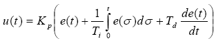
Figure 2-1 shows a diagram of a system with a PID controller. The PID controller compares the measured process value Y with a given reference value Y0. The difference, or error, E, is then processed to calculate a new input process, U. This new input process will attempt to bring the value of the measured process closer to the specified value.

An alternative to a closed loop control system is an open loop control system. An open control loop (without feedback) is not satisfactory in many cases, and its application is often impossible due to the properties of the system.

Figure 2-1. PID closed loop control system

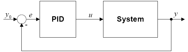
Unlike simple control algorithms, a PID controller is able to control a process based on its history and rate of change. This gives a more accurate and stable control method.

The main idea is that the controller receives information about the state of the system using a sensor. It then subtracts the measured value from the reference value to calculate the error. The error will be handled in three ways: handle the present time by the proportional term, go back to the past using the integral term, and anticipate the future using the differential term.

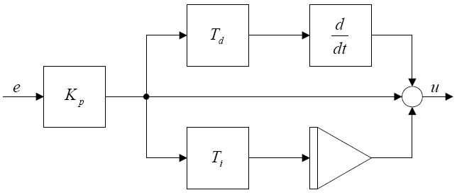
Figure 2-2 shows the circuit diagram of a PID controller, where Tp, Ti, and Td are the proportional, integral, and derivative time constants, respectively.

Figure 2-2. PID Controller Diagram

2.1 Proportional

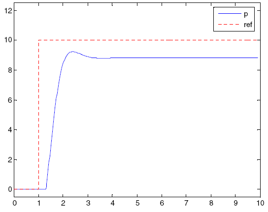
The proportional term (P) gives a control signal proportional to the calculated error. Using only one proportional control always gives a stationary error, except when the control signal is zero and the value of the system process is equal to the required value. On fig. 2-3, a stationary error in the value of the system process appears after a change in the reference signal (ref). Using too large a P-term will give an unstable system.

Figure 2-3. P controller response to a step change in the reference signal

2.2 Integral term

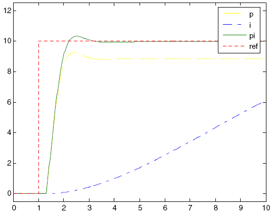
The integral component (I) represents the previous errors. The summation of the error will continue until the value of the system process becomes equal to the desired value. Usually, the integral component is used together with the proportional component, in the so-called PI controllers. Using only the integral component gives a slow response and often an oscillating system. Figure 2-4 shows the step response of the I and PI controllers. As you can see, the response of the PI controller has no stationary error, and the response of the I controller is very slow.

Figure 2-4. The response of the I- and PI controller to a step change in the controlled value

2.3 Derivative term

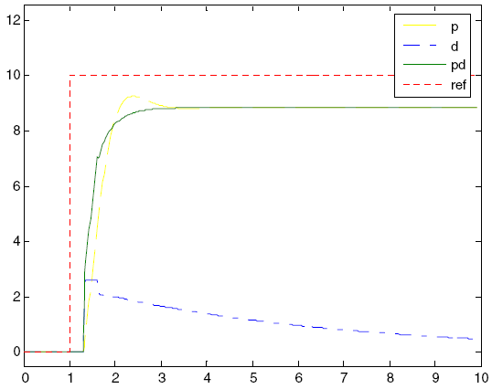
The differential term (D) is the rate of change of the error. The addition of this component improves the response of the system to a sudden change in its state. The differential term D is usually used with P or PI algorithms, like PD or PID controllers. A large differential component D usually gives an unstable system. Figure 2-5 shows the responses of the D and PD controller. The response of the PD controller gives a faster increase in process value than the P controller. Note that the differential term D behaves essentially like a high-pass filter for the error signal and thus easily makes the system unstable and more susceptible to noise.

Figure 2-5. Response of the D- and PD-controller to a step change in the reference signal

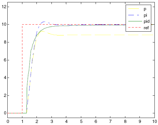
The PID controller gives the best performance because it uses all the components together. Figure 2-6 compares P, PI, and PID controllers. PI improves P by removing the stationary error, and PID improves PI with faster response.

Figure 2-6. P-, PI-, and PID controller response to a step change in the reference signal

2.4. Settings

The best way to find the required parameters of the PID algorithm is to use a mathematical model of the system. However, often there is no detailed mathematical description of the system and the settings of the PID controller parameters can only be made experimentally. Finding parameters for a PID controller can be a daunting task. Here great importance have data about the properties of the system and various conditions her work. Some processes should not allow the process variable to overshoot from the setpoint. Other processes should minimize energy consumption. Also the most important requirement is stability. The process should not fluctuate under any circumstances. In addition, stabilization must occur within a certain time.

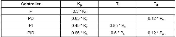
There are some methods for tuning the PID controller. The choice of method will depend largely on whether the process can be offline for tuning or not. The Ziegler-Nichols method is a well-known non-offline tuning method. The first step in this method is to set the I and D gains to zero, increasing the P gain to a steady and stable oscillation (as close as possible). Then the critical gain Kc and the oscillation period Pc are recorded and the P, I and D values ​​are corrected using Table 2-1.

Table 2-1. Calculation of parameters according to the Ziegler-Nichols method

Further parameter tuning is often necessary to optimize the performance of a PID controller. The reader should note that there are systems where a PID controller will not work. These can be non-linear systems, but in general, problems often arise with PID control when the systems are unstable and the effect of the input signal depends on the state of the system.

2.5. Discrete PID controller

The discrete PID controller will read the error, calculate and output the control signal for the sampling time T. The sampling time must be less than the smallest time constant in the system.

2.5.1. Description of the algorithm

Unlike simple control algorithms, the PID controller is able to manipulate the control signal based on the history and rate of change of the measured signal. This gives a more accurate and stable control method.

Figure 2-2 shows the circuit design of the PID controller, where Tp, Ti, and Td are the proportional, integral, and derivative time constants, respectively.

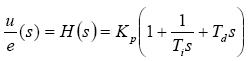
The transfer function of the system shown in Figure 2-2 is:

We approximate the integral and differential components to obtain a discrete form

To avoid this change in the reference process value making any unwanted fast change on the control input, the controller improve based on the derived term on the process values ​​only:

3. Implementation of a PID controller in C

A working C application is attached to this document. A full description of the source code and compilation information can be found in the "readme.html" file.

Figure 3-1. Demo Application Flowchart

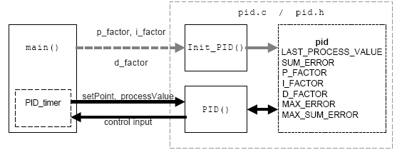
Figure 3-1 shows a simplified diagram of the demo application.

The PID controller uses a structure to store its status and parameters. This structure is initialized by the main function, and only a pointer to it is passed to the Init_PID() and PID() functions.

The PID() function must be called for every time interval T, this is set by a timer that sets the PID_timer flag when the sample time has passed. When the PID_timer flag is set, the main program reads the process reference value and the process system value, calls the PID() function, and outputs the result to the control input.

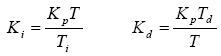
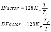
To increase the accuracy, p_factor, i_factor and d_factor are increased by 128 times. The result of the PID algorithm is later reduced by dividing by 128. The value of 128 is used to provide a compilation optimization.

In addition, the influence of Ifactor and Dfactor will depend on the time T.

3.1. Integral windup

When the input process, U, reaches a high enough value, it becomes bounded. Either by the internal numerical range of the PID controller, or by the output range of the controller, or suppressed in the amplifiers. This will happen if there is a big enough difference between the measured value and the reference value, usually because the process has more disturbances than the system is able to handle.

If the controller uses an integral term, this situation can be problematic. In such a situation, the integral term will constantly add up, but in the absence of large violations, the PID controller will begin to compensate the process until the integral sum returns to normal.

This problem can be solved in several ways. In this example, the maximum integral sum is limited and cannot be greater than MAX_I_TERM. Right size MAX_I_TERM will depend on the system.

4. Further development

The PID controller presented here is a simplified example. The controller should work well, but some applications may require the controller to be even more reliable. It may be necessary to add a saturation correction in the integral term, based on the proportional term on the process value only.

In the calculation of Ifactor and Dfactor, the sampling time T is part of the equation. If the sampling time T used is much less than or greater than 1 second, the accuracy of either Ifactor or Dfactor will be insufficient. It is possible to rewrite the PID and scaling algorithm so that the accuracy of the integral and differential terms is preserved.

5. Reference literature

K. J. Astrom & T. Hagglund, 1995: PID Controllers: Theory, Design, and Tuning.
International Society for Measurement and Con.

6. Files

AVR221.rar

Translated by Kirill Vladimirov at the request

Lecture 30Implementation of PID controller and digital filtering in controllers

Microprocessor controllers make it possible to implement both discrete and analog controllers, as well as non-linear and self-tuning controllers. The main problem of digital control is to find the appropriate structure of the controller and its parameters. The software implementation of control algorithms for these parameters is usually a relatively simple task.

Each regulator must also include protection means that prevent the dangerous development of the process under the action of the regulator in emergency situations.

Many TPs are characterized by several input and output parameters. Often the internal connections and interaction of the respective signals are not critical and the process can be controlled with a set of simple controllers, with each loop being used in direct digital control systems.

Linear regulators with one input/output can be represented in a generalized form

Where u is the controller output (control variable), u With is the set value, and at– process output signal (controlled variable). Parameter P represents the order of the regulator.

An ordinary PID controller can be considered as a special case of a generalized discrete controller with P= 2.

Consider a regulator consisting of two parts: a feedback loop (feedback) G Facebook (s) that handles the error E , and feedforward loop G FF (s), which controls changes in the setting action and adds a correction term to the control signal so that the system responds more quickly to changes in the setting. For this controller, the control action U (s ) is the sum of two signals

This expression can be rewritten as

Where U F 1 (s) is a pre-emptive signal based on the reference value (setting action), a U F 2 (s) is a feedback signal.

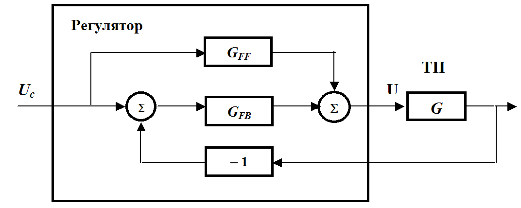
Fig.30.1.A controller containing a feedforward control loop based on a reference value (setpoint) and a feedback loop based on the process output A

The controller has two input signals U c (s) And Y(s) and, therefore, can be described by two transfer functions G F 1 (s) And G R (s).

Since the controller with PF (30.3) has due to G F 1 (s) more adjustable coefficients than a conventional regulator, then the closed control system has better characteristics.

The position of the poles of the feedback system can be changed using the regulator G R (s), and the feedforward controller G F 1 (s) adds new zeros to the system. Therefore, the control system can quickly respond to changes in the task signal if G F 1 (s) is chosen correctly.

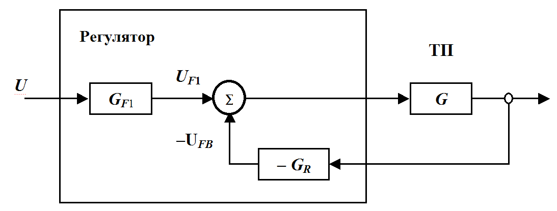
Fig.30.2. Structure of a linear regulator with feedforward control and feedback

Thanks to the use of such a controller, it is possible to create high-precision (servo) control systems by electric drives, robots or machine tools. For them, it is important that the response to the process output is fast and accurate for any change in the reference.

If the numerator and denominator of the PF G R (s), And G F 1 (s) in (23.3) to be expressed by polynomials in s , then the description of the controller after transformations can be represented in the following form

G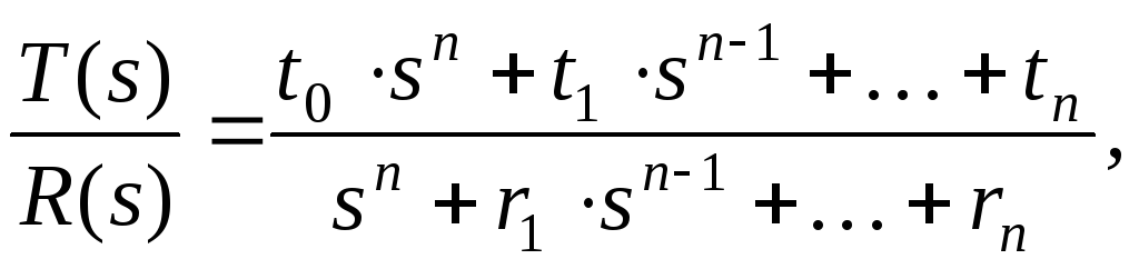



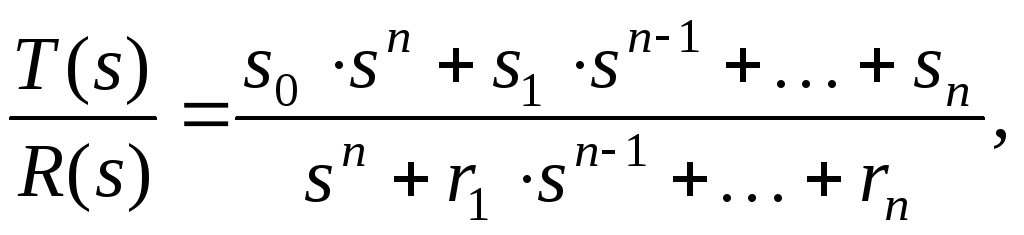de

r i ,s i ,t i – parameters of PF polynomials, s– Laplace operator.

The controller corresponding to equation (30.4) can be represented as a generalized controller (generalcontroller)

The PF of the process can be expressed as

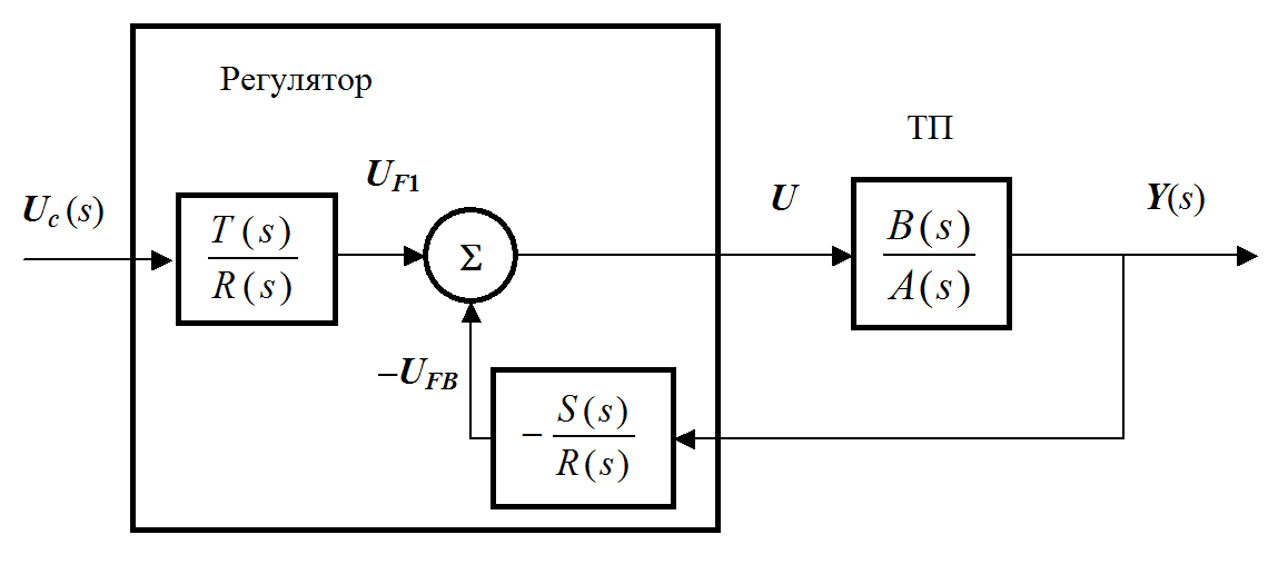
Fig.30.3. The structure of a linear controller with feedforward control and feedback in the form of a PF

If R(s),S(s) And T(s) have a sufficiently high order, i.e., a sufficient number of "tuning knobs", the PF of a closed system can be varied over a wide range. Regulator order P must be the same as the original process. Yes, picking R(s) And S(s), one can arbitrarily change the denominator of the PF of a closed system. Theoretically, this means that the poles of a closed system can be shifted to any place in the complex plane. (In practice, the maximum amplitude and rate of change of the control signal limits the freedom of movement of the poles.)

As a result, an unstable system having a pole with a positive real part can be stabilized with the help of SU.

30.1. PID controller implementation

First of all, a discrete controller model should be developed and an appropriate sampling rate determined. The amplitude of the output value of the regulator must be between the minimum and maximum allowable values. Often it is necessary to limit not only the output signal, but also the rate of change due to the physical capabilities of the MIs and to prevent their excessive wear.

Changing the parameter settings and switching from automatic to manual operation or other changes in operating conditions must not lead to disturbances in the controlled process.

Regulators can be created in analog technology based on operational amplifiers or as digital devices based on microprocessors. However, they have almost the same appearance - a small rugged case that allows installation in an industrial environment.

While digital technology has many advantages, the analog approach is the basis for digital solutions. The advantages of digital controllers include the ability to connect them to each other using communication channels, which allows data exchange and remote control. We are interested in programs for a digital PID controller

Discrete PID controller model . It is necessary for the software implementation of the analog controller. If the controller is designed on the basis of an analog description, and then its discrete model is built, at sufficiently small sampling intervals, time derivatives are replaced by finite differences, and integration is replaced by summation. Process output error is computed for each sample

e(k)=u c (k) – y(k) .

In this case, the sampling interval t s is considered constant, and any signal changes that may have come up during the sampling interval are not taken into account.

There are two types of PID controller algorithm - positional and incremental

Positional PID controller algorithm. In the positional algorithm ( position form) the output signal is the absolute value of the control variable MI. The discrete PID controller has the form

u(k)=u 0 +u P (k)+u I (k)+u D (k).

In this case, the sampling interval ts is considered constant, and any changes in the signal that could come up during the sampling interval are not taken into account.

Even with zero control error, the output signal is non-zero and is determined by the offset u 0 .

The proportional part of the controller has the form

u P (k)= K∙ e(k).

The integral part is approximated by finite differences

u I (k) = u I (k – 1) + K∙ (t s / T i) ∙ e(k)= u I (k – 1) + K∙ a∙ e(k).

The value of the second term at small t s and big T i can become very small, so you need to ensure the required accuracy of its machine representation.

The differential part of the PID controller is approximated by the backward difference

u D (k) =b∙ u D (k – 1) – K∙ (T d / t s) ∙ (1– b)∙ [y(k)– y(k – 1)],

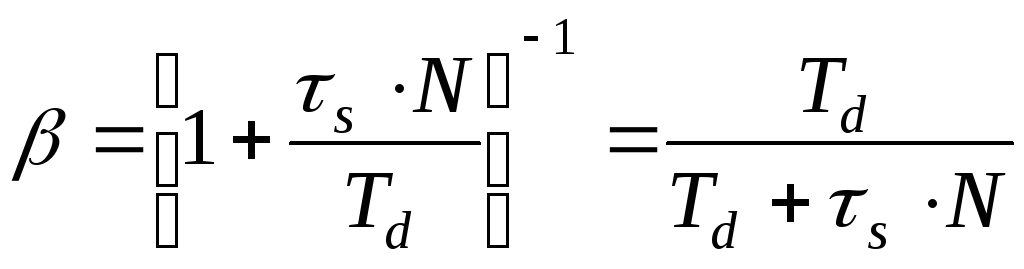
Value T d / N = T f is the normalized N times) the filter time constant in the approximation of the differential component of the control law by an aperiodic link of the first order. Number N taken in the range from 5 to 10. The value b is in the range from 0 to 1.

increment algorithm. It calculates only the change in its output signal. Increment algorithm ( incremental form) The PID controller is convenient to use if the IM is a kind of integrator, such as a stepper motor. Another example of such an MI is a valve whose opening and closing is controlled by impulses and which maintains its position in the absence of input signals.

In the increment algorithm, only changes in the control output signal from the moment of time ( k – 1) until the moment k. The controller algorithm is written as

Δ u I (k) = u (k) – u (k – 1) =Δ u P (k) + Δ u I (k) + Δ u D (k).

The proportional part of the increment algorithm is calculated from the equation

Δ u P (k) = u P (k) – u P (k – 1) =K∙ [e(k)– e(k – 1)] = K∙ Δ e(k).

Integral part - from the equation

Δ u I (k) = u I (k) – u I (k – 1) =K∙ a∙ e(k).

The differential part is from the equation

Δ u D (k) =b Δ u D (k – 1) – K∙ (T d / t s)∙(1– b)∙ [Δ y(k)– Δ y(k – 1),

Δ y(k) =y(k)– y(k – 1).

The algorithm is very simple. For its application, as a rule, operations with a floating point of ordinary precision are sufficient. It does not have problems due to saturation. When switching from manual mode to an automatic regulator that calculates increments, it does not require assigning an initial value to the control signal ( u 0 in the positional algorithm).

The IM can be brought to the desired position during start-up both with manual and automatic control. A small disadvantage of the increment algorithm is the need to take into account the integral component.

The reference value is reduced in both the proportional and differential parts starting from the second sample after it has been changed. Therefore, if a controller based on an incremental algorithm without an integral component is used, the controlled process may drift from the reference value.

Determining the sampling rate in SN . It's more of an art than a science. Too low a sampling rate reduces the efficiency of control, especially the ability of the control system to compensate for disturbances. But if the sampling interval exceeds the process response time, the disturbance can affect the process and disappear before the controller takes corrective action. Therefore, when determining the sampling rate, it is important to take into account both the dynamics of the process and the characteristics of the perturbation.

On the other hand, too high a sampling rate leads to increased computer load and IM wear.

Thus, the determination of the sampling frequency is a compromise between the requirements of process dynamics and the available performance of computers and technological mechanisms. Standard digital controllers operating with a small number of control loops (8 to 16) use a fixed sampling rate on the order of fractions of a second.

The signal-to-noise ratio also affects the sampling rate. At low values ​​of this ratio, i.e. at high noise, a high sampling rate should be avoided, because deviations in the measuring signal are more likely to be associated with high-frequency noise, and not with real changes in the physical process.

An adequate sampling rate is considered to be related to the bandwidth or settling time of the closed loop control system. Rules of thumb recommend that the sampling rate be 6-10 times higher than the bandwidth, or that the settling time be at least five sampling intervals.

In the event that an additional 5-15° phase lag is acceptable, the following rule is valid

t s · ω With = 0,15 – 0,5 ,

where ω With – system bandwidth (at 3 dB level), t s – quantization period, or sampling interval. (This approach is used in many industrial digital single and multi-loop PID controllers.)

Control signal limitation . There are two prerequisites for limiting the control signal:

1) the amplitude of the output signal cannot exceed the range of the DAC at the output of the computer;

2) the operating range of MI is also always limited. The valve does not open more than 100%; the motor cannot be supplied with unlimited current and voltage.

Therefore, the control algorithm must include some function that limits the output signal. In some cases, a deadband, or deadband, must be defined.

If a controller with an incremental algorithm is used, then the changes in the control signal may be so small that the MI cannot process them. If the control signal is sufficient to affect the MI, it is advisable to avoid small but frequent operations, which can accelerate its wear.

A simple solution is to sum small changes in the control variable and issue a control signal MI only after some threshold value has been exceeded. The introduction of a dead zone makes sense only if it exceeds the resolution of the DAC at the output of the computer

Prevention of integral saturation. Integral windup occurs when a PI or PID controller has to compensate for an error that is outside the range of the controlled variable for a long time. Since the output of the regulator is limited, the error is difficult to nullify.

If the control error remains sign for a long time, the value of the integral component of the PID controller becomes very large. This happens if the control signal is limited so much that the calculated output of the regulator differs from the real output of the MI.

Since the integral part only becomes zero some time after the error value has changed sign, integral saturation can lead to large over-shoots. Integral saturation is the result of non-linearities in the system associated with clipping of the output control signal and may never be observed in a linear system.

The influence of the integral part can be limited by conditional integration. As long as the error is large enough, its integral part is not required to form the control signal, but the proportional part is sufficient for control.

The integral part used to eliminate stationary errors is needed only in cases where the error is relatively small. With conditional integration, this component is taken into account in the final signal only if the error does not exceed a certain threshold value. For large errors, the PI controller works like a P controller. Choosing a threshold value for activating the integral term is not an easy task. In analog controllers, conditional integration is performed using a Zener diode (limiter), which is connected in parallel with a capacitor in the feedback circuit of the operational amplifier in the integrating block of the controller. Such a scheme limits the contribution of the integrated signal.

In digital PID controllers, integral saturation is easier to avoid. The integral part is adjusted at each sampling interval so that the controller output does not exceed a certain limit.

The control signal is first calculated using a PI controller algorithm and then checked to see if it exceeds the set limits:

u = u min , If u d < u min ;

u = u d , If u min ≤ u d < u max ;

u = u max , If u d ≤ u max ;

After limiting the output signal, the integral part of the regulator is reset. Below is an example program for a PI controller with saturation protection.

As long as the control signal remains within the set limits, the last statement in the program text does not affect the integral part of the controller.

(*initialization*) c1:=K*taus/Ti;

(*regulator*)

Ipart:= Ipart + c1*e;

ud:=K*e+Ipart; (*calculate control signal*)

if(ud

else if (ud< umax) then u:= ud

Ipart:=u-K*e; (* "anti-saturation" integral part correction *)

An illustration of the problem of integral saturation for a positioning drive with a PI controller is further in fig. 30.4.

Smooth switching of operating modes. When switching from manual to automatic mode, the controller output may jump even if the control error is zero. The reason is that the integral term in the controller algorithm is not always equal to zero. The controller is a dynamic system, and the integral part is one of the elements of the internal state, which must be known when changing the control mode.

The jump in the output value of the controller can be prevented, and the mode change in this case is called a bumpless transition (bumpless transfer).

Two situations are possible: a) transition from manual to automatic mode or vice versa; b) changing the controller parameters.

A smooth transition in case a) for an analog controller is achieved by bringing the process manually to a state in which the measured output value is equal to the reference value.

The process is maintained in this state as long as the controller output is zero. In this case, the integral part is also zero, and since the error is zero, a smooth transition is achieved. This procedure is also valid for digital controllers.

Another method is to slowly bring the reference value to the required final value.

First, the reference value is set equal to the current measurement, and then gradually manually adjusted to the desired value.

If this procedure is performed slowly enough, the integral part of the controller signal remains so small that a smooth transition is ensured. The disadvantage of this method is that it requires a fairly long time, which depends on the nature of the process.

Limiting the rate of change of the control signal . In many control systems, it is necessary to limit both the amplitude and the rate of change of the control signal. For this, special protection circuits are used, connected after the channel for manually entering the reference value. u c (t) and transmitting the filtered signal to the controller u L (t), as shown in Fig. 30.5.

As a result, the process "sees" this control signal instead of the manually entered one. This method is usually used in the regulation of electric drives. Limiting the rate of change of the signal can be achieved with a simple feedback loop.

Hand control signal u c (t), acting as a reference, is compared with a valid control signal u L (t). First, their difference is limited by the limits uemin And uemOh.

The resulting value is then integrated, with the integral being approximated by a finite sum.

The algorithm for limiting the rate of change is as follows:

if (ue< uemin) then uelim:= uemin (*функция ограничения*) else if (ue < uemax) then uelim:= ue

else uelim:= uemax;

uL = uL_old + taus*uelim;

Computational features of the PID controller algorithm. The digital implementation of the PID controller, due to the sequential nature of the calculations, leads to delays that are not found in analog technology. In addition, some limitations (saturation protection and soft transition algorithms) require that the regulator output and the MI pickup occur at the same time. Therefore, computational delays must be kept to a minimum. To do this, some elements of the digital regulator are calculated before the sampling time.

For a regulator with saturation protection, the integral part can be calculated in advance using forward differences

u I (k + 1) =u I (k)+c 1 · e (k) + c 2 · [u (k) – u d (k) ] ,

Where u – limited value u d ;

T t is a coefficient called the tracking time constant.

The differential part looks like

c 3 = (1– b) · K· T d /t s ;

x (k- 1) = b· u D (k- 1)+c 3 · y (k- 1).

variable x can be updated immediately after the point in time k

x (k) = b· x(k- 1)+c 3 (1 – b) · y (k).

Thus, u D (k + 1) can be calculated from (24.2) as soon as the measurement result is obtained y(k + 1).

Optimization of the calculations is necessary, since the digital regulator sometimes has to perform several thousand control operations per second. Under these conditions, it is important that some coefficients are available immediately, rather than being recalculated each time. In addition, industrial regulators do not have the fastest processors ( i 386, 486). Therefore, the order and type of calculations greatly affect the speed of control operations.

PID algorithm . An example of a PID controller program in Pascal. Calculation of coefficients c 1 ,c 2 and c 3 must be done only if the controller parameters are changed K, T i , T d And T f. The controller algorithm is executed at the time of each sample. The program has protection against saturation of the integral component.

(*Precalculation of coefficients*)

c1:=K*taus / Ti; (* Equation 23.7 *)

с2:= taus / Tt; (* Equation 24.1 *)

beta:=Td / (Td+taus*N); (* Equation 24.1 *)

c3:= K*Td*(l-beta) / taus; (* Equation 24.2 *)

c4:= c3*(1 - beta); (* local constant*)

(* Control algorithm *)

uc:=ADinput(ch1); (* reference value input, analog input *)

y:= AD_input(ch2); (* measurement input, analog input *)

e:= uc-y; (* control error calculation *)

ppart:= K*e; (*proportional part*)

dpart:= x - (c3*y); (* differential part, *)

ud:=uO+ppart+ipart+dpart; (* regulator output before clipping*)if(ud

Send your good work in the knowledge base is simple. Use the form below

Students, graduate students, young scientists who use the knowledge base in their studies and work will be very grateful to you.

Hosted at http://www.allbest.ru

Ministry of Education and Science of the Russian Federation

Federal State Budgetary Educational Institution

higher professional education

"KUBAN STATE UNIVERSITY"

(FGBOU VPO "KubGU")

BACHELOR'S FINAL QUALIFICATION WORK

Development and design of PID controllers

The work was done by Roman Valerievich Presnyakov

Scientific director

dr. Phys.-Math. sciences, professor

E.N. Tumaev

Comptroller

cand. Phys.-Math. Sciences, Associate Professor A. A. Martynov

Krasnodar 2015

Final qualifying work 83 pages, 29 pictures, 42 sources.

PID CONTROL, EMBEDDED SYSTEMS, MICROCONTROLLERS, SOFTWARE MODULES, MSP430, INTERRUPT

The object of study of the final qualification work is the study of the general principles of building proportional-integral-differential technological controllers and designing an algorithm for temperature controllers based on cheap MSP430 microcontrollers (Texas Instruments). The paper provides an overview of the means of modern microcontrollers and the principles of their operation.

The analysis of the problems of hardware and software implementation of technological microprocessor controllers is carried out. Recommendations are given for the design of microprocessor-based measuring and control instruments and the creation of software for embedded systems. A variant of the implementation of the PID controller algorithm is proposed. A distinctive feature is the use of algorithms that exclude the use of floating point numbers.

Designations and abbreviations

Introduction

2. Sensitivity functions. Digital Pid Equation

2.2 Discrete form of the controller. Digital PID Equation

3. Regulatory quality

3.1 Weakening of the influence of external disturbances. Quality Criteria

4. Setting the controller parameters. basic principles

4.1 Selection of controller parameters. Manual and Auto settings

5. Embedded systems programming

5.1 General principles for the development of embedded systems

5.2 Stages of creating software for embedded systems

5.3 Hierarchy of executable code in embedded systems

6. Algorithm of the created software

6.1 Description of the operation algorithm of the PID temperature controller based on the MSP430F149 microcontroller

Conclusion

List of sources used

Designations and abbreviations

temperature controller microcontroller

	microcontroller
PID algorithm	Proportional-integral-differential algorithm
	hardware abstraction layer (hardware abstraction layer)
	Integrated development environment (integrated development environment)
	pulse width modulation
	programmable logic controller
	supervisory control and data acquisition (supervisory control and data acquisition)
	serial peripheral interface (serial peripheral interface)
	application programming interface (application programming interface)
	automated workplace
	software

INTRODUCTION

The control of technological processes with the help of controllers operating according to the proportional-integral-differential law (PID controllers) allows maintaining the required technological value with a sufficiently high accuracy and acceptable noise immunity to external disturbing influences. Modern PID controllers are implemented both as a software module of a SCADA system executed at an automated workstation (AWS) or a programmable logic controller (PLC), and as separate process controllers located on local and central control cabinets. As the basic elements of information processing and control, microprocessors with limited functionality are often used, which raises the problem of a lack of hardware resources and an increase in the cost of the system.

The purpose of this work is to review the principles of building proportional-integral-derivative controllers and to develop, on the basis of the review, the principles for creating a temperature PID controller.

When creating a temperature PID controller, a programmable microprocessor technological meter-regulator F0303.2 based on the MSP430F149 microcontroller, MSP-FET430UIF programmer, P3003 voltage comparator with a voltage output range from 10 nV to 11.111110 V and an accuracy class of 0.0005 were used. The microcontroller program was created in the IAR Embedded Workbench for MSP430 6 integrated development environment. The technical documentation was obtained from the website of the microcontroller manufacturer.

For the full implementation of PID control in a microprocessor device, it is necessary to implement the following subsystems:

Measurement subsystem

PID Algorithm Processing Subsystem

Management User Interface Subsystem

Regulatory impact output subsystem

1. Principles of creating PID controllers

1.1 General issues of implementing PID controllers

For practical implementation, it is necessary to take into account the features generated by the real conditions of application and technical implementation. These features include:

Finite dynamic range of changes in physical variables in the system (eg limited heater power, limited valve capacity);

It is not always possible to change the sign of the control action (for example, there is often no refrigerator in the temperature maintenance system, the engine may not have a reverse stroke, not every aircraft has a negative thrust system);

Limited measurement accuracy, which requires special measures to perform the differentiation operation with an acceptable error;

The presence of typical non-linearities in almost all systems: saturation (limiting the dynamic range of variable changes), limiting the slew rate, hysteresis and backlash;

Technological dispersion and random variations of the parameters of the controller and the object;

Discrete implementation of the controller;

The need for smooth (shockless) switching of control modes;

1.2 PID Derivative Assembly

The problem of numerical differentiation is quite old and common in both digital and analog controllers. Its essence lies in the fact that the derivative is usually calculated as the difference between two variables of close magnitude, so the relative error of the derivative always turns out to be greater than the relative error of the numerical representation of the differentiable variable.

In particular, if the input of the differentiator receives a sinusoidal signal A * sin (sht), then at the output we get A * w * cos (sht), that is, with increasing frequency w, the amplitude of the signal at the output of the differentiator increases. In other words, the differentiator amplifies high-frequency interference, short bursts, and noise.

If the interference amplified by the differentiator lies outside the operating frequency range of the PID controller, then they can be attenuated using a high-pass filter. The structural implementation of a differentiator with a filter is shown in Figure 1. Here

that is, the transfer function of the resulting differentiator D(s) can be represented as the product of the transfer function of an ideal differentiator and the transfer function of a first-order filter:

where the coefficient N sets the cutoff frequency of the filter and is usually chosen equal to 2…20;

T/N -- filter time constant;

s is the complex frequency.

Greater high-frequency noise attenuation can be obtained with a separate filter that is connected in series with the PID controller. Usually a second-order filter with a transfer function is used

The filter time constant is chosen equal to TF = Ti/N, where N = 2…20, Ti is the integration constant of the PID controller. It is advisable not to choose the cutoff frequency of the filter below the frequency 1/Ti, since this complicates the calculation of the controller parameters and the stability margin.

Figure 1 - Structural implementation of the differential term of the PID controller

In addition to differentiation noise, the performance of the PID controller is affected by measurement noise. Through the feedback loop, these noises enter the system input and then appear as the dispersion of the control variable u. High-frequency noise is harmful because it causes accelerated wear of pipeline fittings and electric motors.

Because the control object is usually a low-pass filter, measurement noise rarely travels through the control loop to the system output. However, they increase the measurement error y(t) and reduce the accuracy of regulation.

In PID controllers, noise with a spectrum in the low-frequency region, caused by external influences on the control object, and high-frequency noise associated with electromagnetic interference, noise on the power and ground buses, with sampling of the measured signal, and other reasons are distinguished. Low-frequency noise is modeled as an external disturbance d(s), high-frequency noise is modeled as measurement noise n(s).

1.3 Integral node of the PID controller. integral saturation

In steady state operation and with small disturbances, most systems with PID controllers are linear. However, the process of entering the regime almost always requires taking into account the nonlinearity of the “limitation” type. This non-linearity is due to natural limitations on power, speed, rpm, angle of rotation, valve cross-sectional area, dynamic range, etc. The control loop in a system that is in saturation (when the variable has reached the limit) turns out to be open, since when the variable at the input of the link with the limit changes, its output variable remains unchanged.

The most typical manifestation of the limitation mode is the so-called "integral saturation", which occurs when the system reaches the mode in controllers with a nonzero integration constant Ti? 0. Integral saturation leads to a delay in the transient process (Figures 2 and 3). A similar effect occurs due to the limitation of the proportional and integral term of the PID controller (Figures 4 and 5). However, integral saturation is often understood as a set of effects associated with a nonlinearity of the “limitation” type.

T 1= 0.1 s; T2 =0.05 s; L = 0.02 s; K = 2; Ti = 0.06 s; Td = 0

Figure 2 - The response of the output variable y(t) to the jump in the input action r(t) for the PI controller under the condition of limiting the power at the input of the object u(t) and without limitation (second order object)

T1 = 0.1 s; T2 = 0.05 s; L = 0.02 s; K = 2; Ti = 0.06 s; Td = 0

Figure 3 - Signal at the input of the object u(t) with and without power limitation (second order object)

K = 10; Ti = 0.014 s; Td = 0.3 s; T1 = 0.1 s; T2 = 0.05 s; L = 0.02 s

Figure 4 - The response of the output variable y(t) to the jump in the input action r(t) for the PID controller under the condition of limiting the power at the input of the object u(t) and without limitation (second order object)

T1 = 0.1 s; T2 = 0.05 s; L = 0.02 s; K = 10; Ti = 0.014 s; Td = 0.3 s

Figure 5 - The signal at the input of the object u(t) in the loop with the PID controller under the condition of power limitation and without (second order object)

and second order

where Kp is the transfer coefficient in steady state;

T, T1, T2 - time constants;

L - transport delay.

The essence of the problem of integral saturation is that if the signal at the input of the control object u(t) has entered the saturation (limitation) zone, and the mismatch signal r(t) - y(t) is not equal to zero, the integrator continues to integrate, that is, the signal increases at its output, but this signal does not participate in the regulation process and does not affect the object due to the saturation effect. The control system in this case becomes equivalent to an open system, the input signal of which is equal to the saturation level of the control signal u(t).

For thermal systems, the lower limit is usually zero heating power, while the PID controller requires a “negative heating power” to be applied to the object, that is, cooling the object. The effect of integral saturation has been known for a long time. In analog regulators, its elimination was quite difficult, since in them the problem could not be solved algorithmically, but was solved only by hardware.

With the advent of microprocessors, the problem can be solved much more efficiently. Methods for eliminating integral saturation are usually the subject of inventions, belong to the trade secret of manufacturing companies and are protected by patents.

Limiting the slew rate of the input action. Since the maximum value of the input action on the control object u(t) decreases with a decrease in the difference r(t) - y(t), then to eliminate the limitation effect, you can simply reduce the slew rate of the setpoint signal r(t), for example, using a filter. The disadvantage of this method is the reduction in system speed, as well as the inability to eliminate the integral saturation caused by external disturbances, and not by the setpoint signal.

When the control action on the object reaches saturation, the feedback breaks and the integral component continues to grow, even if it should have fallen in the absence of saturation. Therefore, one of the methods to eliminate the integral saturation is that the controller monitors the magnitude of the control action on the object, and as soon as it reaches saturation, the controller enters a software prohibition of integration for the integral component.

Saturation compensation with additional feedback. The effect of integral saturation can be weakened by monitoring the state of the actuator entering saturation and compensating the signal applied to the input of the integrator. The structure of a system with such a compensator is shown in Figure 6.

Figure 6 - Compensation for the effect of integral saturation with the help of additional feedback for transmitting the error signal es to the input of the integrator

The principle of its work is as follows. The system generates a mismatch signal between the input and output of the actuator es = u - v. The signal at the output of the actuator is either measured or calculated using a mathematical model (Figure 6). If es = 0, this is equivalent to no compensator and we get a normal PID controller. If executive device saturates, then v > u and es< 0. При этом сигнал на входе интегратора уменьшается на величину ошибки es, что приводит к замедлению роста сигнала на выходе интегратора, уменьшению сигнала рассогласования и величины выброса на переходной характеристике системы (рисунки 7 и 8). Постоянная времени Ts определяет степень компенсации сигнала рассогласования.

Figure 7 - System response to a single jump r(t) for different values ​​of the time constant Ts

K = 7; Ti = 0.01 s; Td = 0.1 s; T1 = 0.1 s; T2 = 0.05 s; L = 0.01 s

Figure 8 - System response to the error signal es (second-order object, controller parameters:

In some controllers, the input u of the comparator es is singled out as a separate input - the “tracking input”, which is convenient when building complex control systems and when cascading several controllers.

Conditional integration. This method is a generalization of the algorithmic prohibition of integration. After the onset of the prohibition, the integral component remains constant, at the same level that it had at the moment the integration prohibition appeared. The generalization is that the prohibition of integration occurs not only when saturation is reached, but also under certain other conditions.

Such a condition can be, for example, the achievement by the error signal e or the output variable y of a certain specified value. When turning off the integration process, it is necessary to monitor the state of the integrator at the moment of turning it off. If it accumulates an error and the degree of saturation increases, then the integration is turned off. If, at the moment of switching off, the degree of saturation decreases, then the integrator is left on.

Figure 9 shows an example of a transient process in a system with the integrator turned off when the output value y(t) reaches a given value (y = 0, y = 0.2, y = 0.8).

Figure 9 - Response to a single jump r(t) of a system with actuator saturation at various integrator shutdown levels y

Constrained Integrator. In a variant of the implementation of the PI controller using an integrator in the feedback loop was presented. If this circuit is supplemented with a limiter (Figure 10), then the signal u at the output will never go beyond the limits set by the limiter thresholds, which reduces the overshoot in the transient response of the system (Figure 12). Figure 11 shows a modification of such a limiter.

The model of the clipping effect can be improved if, after exceeding the level at which the clipping occurs, the signal at the output of the model is reduced (Figure 13). This accelerates the recovery of the system from saturation mode.

Figure 10 - Modification of the integrator with a limiter (in parallel)

Figure 11 - Modification of the integrator with a limiter (in series)

Figure 12 - Response to a single jump r(t) of a system containing

integrator with upper constraint Uup

Figure 13 - Improved transfer function of clipping effect model

1.4 Margin of stability of the system. Nyquist criterion

The possibility of loss of stability is the main disadvantage of feedback systems. Therefore, ensuring the necessary stability margin is the most important step in the development and tuning of the PID controller.

The stability of a system with a PID controller is the ability of the system to return to tracking the setpoint after the cessation of external influences. In the context of this definition, external influences mean not only external disturbances acting on the object, but any disturbances acting on any part of the closed system, including measurement noise, temporal setpoint instability, sampling and quantization noise, noise and calculation error. All these perturbations cause deviations of the system from the equilibrium position. If

after the termination of their influence, the system returns to the equilibrium position, then it is considered stable. When analyzing the stability of PID controllers, it is usually limited to studying the response of the system to a step change in the setpoint r(t), measurement noise n(t) and external disturbances d(t). The loss of stability manifests itself as an unlimited increase in the controlled variable of the object or as its oscillation with increasing amplitude.

In production conditions, attempts to achieve the stability of a system with a PID controller empirically, without its identification, do not always lead to success (first of all, this applies to systems with a high-order object or objects that are difficult to identify, as well as systems with a large transport delay) . It seems that stability is a mystical property that cannot always be controlled. However, if the process is identified accurately enough, then the mysticism disappears and the stability analysis is reduced to the analysis of a differential equation describing a closed loop with feedback. Of practical interest is the analysis of the stability margin, that is, the determination of the numerical values ​​of the criteria that allow you to indicate how far the system is from the state of instability.

The most complete information about the stability margin of the system can be obtained by solving a differential equation that describes a closed system under external disturbances. However, this process is too time-consuming, therefore, for linear systems, simplified methods are used to estimate the stability margin without solving equations. We will consider two estimation methods: using the hodograph of the complex open-loop frequency response (Nyquist criterion) and using the logarithmic frequency response and phase response (Bode plots).

A stable system can become unstable with small changes in its parameters, for example, due to their technological dispersion. Therefore, further we will analyze the sensitivity function of a system with a PID controller, which allows us to identify the conditions under which the system becomes coarse (insensitive to changes in its parameters). A system that maintains a given stability margin over the entire range of parameter changes due to their technological variation, aging, operating conditions, over the entire range of load parameter changes, as well as over the entire range of disturbances acting on the system in real operating conditions, is called robust. Sometimes robustness and rudeness are used as equivalent concepts.

Nyquist criterion. Consider a system consisting of a controller R and a control object P (Figure 14), which is obtained by eliminating the setpoint signal circuit from a classical system with a PID controller. We will assume that the feedback is open, and to close it, it is enough to connect the points x and y. Suppose now that the input x is given a signal

Then, having passed through the controller and the control object, this signal will appear at the output y with a changed amplitude and phase in the form:

y(t) = ? |G(jw0)|sin(w0t + ?), (4)

where G(jsh) = R(jsh)P(jsh) is the complex frequency response (CFC) of the system, ? = arg(G(jш0)) - CCH argument, |G(jш0)| - CFC module at frequency w0. Thus, when passing through the regulator and the object, the signal amplitude will change in proportion to the modulus, and the phase - by the value of the CFC argument.

Figure 14 - Structure of an open-loop control system with a PID controller for stability analysis

If we now close the points x and y, then the signal will circulate in a closed loop, and the condition y(t) = x(t) will be satisfied. If, in addition, |G(jш0)| ? 1 and? \u003d 180 °, that is, after passing through the loop, the signal enters the controller input in the same phase as in the previous cycle, then after each passage through the loop, the amplitude of the sinusoidal signal will increase until it reaches the boundary of the system linearity range, after which the oscillation shape becomes different from sinusoidal. In this case, the harmonic linearization method can be used to analyze the stability, when only the first harmonic of the distorted signal is considered. In the steady state, after the oscillation amplitude is limited, due to the equality y(t) = x(t), the following condition will be satisfied:

|G(jw0)|=1, i.e. G(jw0)= - 1 (5)

By solving the equation G(jw0) = -1, you can find the frequency of oscillations w0 in a closed system.

The complex frequency response G(jш) is graphically depicted in the form of a hodograph (Nyquist diagram) - a graph in the coordinates Re and Im (Figure 15). The arrow on the hodograph line indicates the direction of movement of the "pencil" with increasing frequency. The point G(jw0) = -1, which corresponds to the condition for the existence of undamped oscillations in the system, on this graph has the coordinates Re = -1 and Im = 0. Therefore, the Nyquist stability criterion is formulated as follows: a circuit that is stable in the open state will remain stable and after its closure, if its CFC in the open state does not cover the point with coordinates [-1, j0]. More strictly, when moving along the hodograph trajectory in the direction of increasing frequency, the point [-1, j0] must remain on the left so that the closed loop is stable.

K=6; T1 = T2 = 0.1 s; L = 0.01 s

Figure 15 - Three hodographs of the CFC of an open system G(jw) for a second-order object

Figure 16 shows the responses of a closed system with three different hodographs (Figure 15) to a single setpoint step. In all three cases, the system is stable, but the damping rate of oscillations and the shape of the transition

their process is different. It is intuitively clear that a system with parameters Ti = 0.01 s, Td = 0.1 s is closest to going into a state of undamped oscillations with a small change in its parameters. That's why

when designing a PID controller, it is important to ensure not so much stability as its reserve, which is necessary for the normal functioning of the system in real conditions.

The stability margin is estimated as the degree of remoteness of the CFC from the critical point [-1, j0]. If |G(jш0)|< 1, то можно найти, во сколько раз осталось увеличить передаточную функцию, чтобы результирующее усиление вывело систему в колебательный режим: gm|G(jщ0)| = 1, откуда

The gain margin gm is the value by which the transfer function of an open-loop system G(jsh180) must be multiplied so that its module at a phase shift frequency of 180 ° (sh180) becomes equal to 1. If at a frequency of w180 the open loop gain is G(jsh180) = -1/gm (Fig. 15), then an additional gain of gm will bring the system to the point [-1, j0], since (-1/gm) gm = -1. The concept of phase margin is introduced similarly: this is the minimum value m by which it is necessary to increase the phase shift in an open system arg(G(jw)) so that the total phase shift reaches 180°, that is

The “+” sign before arg(G(jш1)) is because arg(G(jш1))< 0. Для оценки запаса устойчивости используют также минимальное расстояние sm от кривой годографа до точки [-1, j0] (рисунок 15).

In practice, the values ​​gm = 2...5,m = 30...60°, sm = 0.5...0.8 are considered acceptable. For the graph in Figure 15, these criteria have the following values:

Gm1 = 12.1; m1 = 15°; sm1 = 0.303 (for the case Ti = 0.01 s,

Gm2 = 11.8; m2 = 47.6°; sm2 = 0.663 (for the case Ti = 0.05 s,

Gm3 = 1.5; m3 = 35.2°; sm3 = 0.251 (for the case Ti = 0.05 s,

If the hodograph curve intersects the real axis at several points, then to assess the stability margin, take the one that is closest to the point [-1, j0]. With a more complex hodograph, an estimate of the stability margin as a delay margin can be used. The delay margin is the minimum delay added to the loop to make it unstable. Most often, this criterion is used to assess the stability margin of systems with the Smith predictor.

Frequency stability criterion. For a graphical representation of the transfer function of an open system and an assessment of the stability margin, logarithmic frequency response and phase response can be used (Figure 17). To assess the phase margin, first, using the frequency response, the frequency u1 (cutoff frequency, or unity gain frequency) is found, at which G(ju1) = 1, then the corresponding phase margin is found from the PFC. To estimate the gain margin, first, using the PFC, find the frequency w180, at which the phase shift is 180 °, then find the gain margin from the frequency response. Figure 17 shows examples of graphical constructions for estimating the gain and phase margin for the system, the hodographs of which are shown in Figure 15.

If the open loop phase margin is 0° or the gain margin is 1, the system will be unstable after the feedback loop is closed.

Figure 16 - Transient response of a closed system, which

has hodographs shown in Figure 15

2. Sensitivity functions. digital PID controller equation

2.1 Sensitivity functions. robustness. Shockless switching of control modes

The transfer function of a real object P(s) can change during operation by the value DP(s), for example, due to changes in the load on the motor shaft, the number of eggs in the incubator, the level or composition of the liquid in the autoclave, due to aging and wear of the material, the appearance of backlash, lubrication changes, etc. A properly designed automatic control system should maintain its quality indicators not only in ideal conditions, but also in the presence of the listed harmful factors. To assess the influence of a relative change in the transfer function of the object DP / P on the transfer function of the closed system Gcl

y(s) = r(s), Gcl(s) = (8)

find the differential dGcl:

Dividing both sides of this equality by Gcl and substituting Gcl = PR/(1+PR) into the right side, we get:

Figure 17 - Evaluation of the gain and phase margin for a system with a hodograph shown in Figure 15

From (10) the meaning of the coefficient S is visible - it characterizes the degree of influence of the relative change in the transfer function of the object on the relative change in the transfer function of the closed loop, that is, S is the coefficient of sensitivity of the closed loop to the variation in the transfer function of the object. Since the coefficient S \u003d S (jsh) is frequency dependent, it is called the sensitivity function.

As follows from (10),

Let's introduce the notation:

The value T is called the complementary (additional) sensitivity function, since S + T = 1. The sensitivity function allows you to evaluate the change in the properties of the system after the feedback is closed. Since the transfer function of an open system is equal to G = PR, and of a closed system Gcl = PR/(1+PR), then their ratio is Gcl/G = S. Similarly, for an open system, the transfer function from the input of disturbances d to the output of a closed system is (see ) P(s)/(1 + P(s)R(s)), and open-loop is P(s), so their ratio is also S. For the transfer function from the measurement noise input n to the system output, the same ratio can be obtained S.

Thus, knowing the form of the function S(jw) (for example, Figure 18), we can say how the suppression of external influences on the system will change for different frequencies after the feedback loop is closed. Obviously, the noises lying in the frequency range in which |S(jш)| > 1, after closing the feedback will increase, and the noise with frequencies at which |S(jш)|< 1, после замыкания обратной связи будут ослаблены.

The worst case (the greatest amplification of external influences) will be observed at the maximum frequency Ms of the modulus of the sensitivity function (Figure 18):

The maximum of the sensitivity function can be related to the stability margin sm (Figure 15). For this, we pay attention to the fact that |1 + G(jш)| represents the distance from the point [-1, j0] to the current point on the hodograph of the function G(jш). Therefore, the minimum distance from the point [-1, j0] to

function G(jш) is equal to:

Comparing (13) and (14), we can conclude that sm = 1/Ms. If the module G(jsh) decreases with increasing frequency, then, as can be seen from Figure 15, (1-sm) ? 1/gm. Substituting here the ratio sm = 1/Ms, we obtain an estimate of the gain margin expressed in terms of the maximum of the sensitivity function:

Similarly, but with coarser assumptions, we can write the phase margin estimate in terms of the maximum of the sensitivity function :

For example, for Ms = 2 we get gm ? 2 and? 29°.

Figure 18 - Sensitivity functions for the system with hodographs shown in Figure 13

Robustness is the ability of a system to maintain a given stability margin with variations in its parameters caused by a change in load (for example, when the furnace load changes, its time constants change), technological spread of parameters and their aging, external influences, calculation errors and object model error. Using the concept of sensitivity, we can say that robustness is a low sensitivity of the stability margin to variations in the parameters of an object.

If the parameters of the object change within small limits, when it is possible to use the replacement of the differential with a finite increment, the effect of changes in the parameters of the object on the transfer function of the closed system can be estimated using the sensitivity function (10). In particular, it can be concluded that at those frequencies where the modulus of the sensitivity function is small, the effect of changes in the object parameters on the transfer function of a closed system and, accordingly, on the stability margin will be small.

To assess the impact of large changes in the parameters of the object, we represent the transfer function of the object in the form of two terms:

P = P0 + DP, (17)

where P0 is the calculated transfer function, DP is the deviation from P0, which must be a stable transfer function. Then the loop gain of an open system can be represented as G = RP0 + RDP = G0 + RDP. Since the distance from the point [-1, j0] to the current point A on the hodograph of the unperturbed system (for which DP = 0) is equal to |1 + G0| (Figure 19), the stability condition for a system with loop gain deviation RDP can be represented as:

|RDP|< |1+G0|,

where T is an additional sensitivity function (12). Finally, we can write the ratio:

which must be fulfilled in order for the system to remain stable when the process parameters change by the value of DP(jsh).

Reduction of zeros and poles. Since the open-loop transfer function G = RP is the product of two transfer functions, which in general case have both a numerator and a denominator, then it is possible to cancel the poles that lie in the right half-plane or are close to it. Since in real conditions, when there is a spread of parameters, such a reduction is performed inaccurately, a situation may arise when a theoretical analysis leads to the conclusion that the system is stable, although in fact, with a small deviation of the process parameters from the calculated values, it becomes unstable.

Therefore, every time when the poles are reduced, it is necessary to check the stability of the system with a real scatter of the object's parameters.

Figure 19 - Explanation of the derivation of the ratio (18)

The second effect of the shortening of the poles is the appearance of a significant difference between the settling time of the transient process in a closed system under the influence of a setpoint signal and external disturbances. Therefore, it is necessary to check the response of the synthesized controller under the influence of not only the setpoint signal, but also external disturbances.

Shockless switching of control modes. In PID controllers, there may be modes when their parameters change abruptly. For example, when it is necessary to change the integration constant in a running system or when, after manual control of the system, it is necessary to switch to automatic mode. In the cases described, undesirable overshoots of the controlled variable may occur if special measures are not taken. Therefore, the problem arises of smooth (“shockless”) switching of operating modes or controller parameters. The main method of solving the problem is to build such a controller structure, when the parameter change is performed before the integration stage. For example, with a changing parameter Ti = Ti (t), the integral term can be written in two forms:

I(t) = or I(t) = .

In the first case, when Ti (t) changes abruptly, the integral term will change abruptly, in the second case, it will change smoothly, since Ti (t) is under the integral sign, the value of which cannot change abruptly.

A similar method is implemented in the incremental form of the PID controller (see section "Incremental form of the digital PID controller") and in the serial form of the PID controller, where the integration is performed at the final stage of the control calculation.

2.2 Discrete controller form Digital PID controller equation

Continuous variables are convenient to use for the analysis and synthesis of PID controllers. For technical implementation, it is necessary to switch to a discrete form of equations, since the basis of all controllers is a microcontroller, controller or computer that operates with variables obtained from analog signals after their time quantization and level sampling.

Due to the finite time for calculating the control action in the microcontroller and the delay in analog-to-digital conversion between the moment the analog signal arrives at the input of the controller and the appearance of the control action at its output, an undesirable delay appears, which increases the overall delay in the control loop and reduces the stability margin.

The main effect that appears during sampling and which is often "rediscovered" is the appearance of alias frequencies in the spectrum of the quantized signal in the case when the quantization frequency is not high enough.

A similar effect occurs when filming a spinning car wheel. The frequency of the alias signal is equal to the difference between the interference frequency and the quantization frequency. In this case, the high-frequency interference signal is shifted to the low-frequency region, where it is superimposed on the useful signal and creates big problems, since it is impossible to filter it at this stage.

To eliminate the alias effect, it is necessary to install an analog filter before the input of the analog-to-digital converter, which would attenuate the noise by at least an order of magnitude at a frequency equal to half the quantization frequency. Usually a Butterworth filter of the second or higher order is used. The second solution to the problem is to increase the quantization frequency so that it is at least 2 times (according to the Kotelnikov theorem) higher than the maximum frequency of the interference spectrum. This allows a digital low-pass filter to be applied after quantization. With such a sampling rate, the received digital signal is completely equivalent to the analog one in terms of the amount of information, and all the properties of the analog controller can be extended to the digital one.

Transition to finite-difference equations. The transition to discrete variables in the analog controller equations is performed by replacing derivatives and integrals with their discrete counterparts. If the equation is written in operator form, then first a transition is made from the image area to the original area. In this case, the differentiation operator is replaced by a derivative, the integration operator is replaced by an integral.

There are many ways to approximate derivatives and integrals by their discrete counterparts, which are outlined in courses on numerical methods for solving differential equations. In PID controllers, the most common are the simplest types of approximation of the derivative by a finite difference and the integral by a finite sum. Consider the integral term of the PID controller:

Differentiating both parts with respect to time, we get

Replacing the differentials in this expression with finite differences (left differences), we obtain

where the index i means that the given value was taken at time ti (note that here and below the index i in Ti denotes not the number of the time step, but integral coefficient PID controller). From the last expression we get:

Thus, the next value of the integral can be calculated knowing the previous one and the value of the error at the previous time. However, such a formula tends to accumulate a calculation error over time if the ratio Dt/Ti is not small enough. Another integration formula is more stable - with right differences, when the error value is taken at the same time as the calculated integral:

Consider the differential term of a PID controller with a filter:

Passing in this formula from images to originals, we get:

Replacing the differentials with finite increments, we obtain the difference equation:

Note that for the convergence of the iterative process (21) it is necessary that

When Dt > Td/N, the iterative process (21) becomes oscillatory, which is unacceptable for the PID controller. The difference equation obtained using the right differences has the best characteristics:

Here, the convergence condition is satisfied for all Dt, and no oscillations occur for any values ​​of the parameters. In addition, the last formula allows you to “turn off” the differential component in the PID controller by setting Td = 0, which cannot be done in expression (21), since division by zero occurs in this case. You can use even more precise formulas for numerical differentiation and integration, known from the course of numerical methods for solving equations. The value of the quantization cycle Dt is chosen as small as possible, this improves the quality of regulation. To ensure good quality of regulation, it should not be more than 1/15...1/6 of the time of establishing the transient response of the object at the level of 0.95 or 1/4...1/6 of the value of the transport delay. However, with an increase in the quantization frequency by more than 2 times compared with the upper frequency of the spectrum of disturbing signals (according to the Kotelnikov theorem), there is no further improvement in the quality of regulation.

If there is no anti-alias filter at the regulator input, then the quantization frequency is chosen 2 times higher than the upper cutoff frequency of the noise spectrum in order to use digital filtering. It should also be taken into account that the executive device must have time to work out during the time Dt.

If the controller is used not only for regulation, but also for alarm signaling, then the quantization cycle cannot be less than the allowable delay for the operation of the alarm signal.

With a small quantization cycle, the error in calculating the derivative increases. To reduce it, you can use the smoothing of the received data on several collected points before the differentiation stage.

Digital PID controller equation. Based on the above, the discrete PID controller equation can be written as:

where i is the number of the time step.

To start the algorithm, we usually choose uD0 = 0, I0 = 0, e0 = 0, but there may be others initial conditions, depending on the meaning of a specific control problem.

Note that the algorithm obtained by simply replacing the differentiation and integration operators in the classical PID controller equation

end differences and end sums

has poor stability and low accuracy, as shown earlier. However, as the sampling frequency increases, the difference between the above two algorithms is erased.

Incremental form of a digital PID controller. Quite often, especially in neural network and fuzzy controllers, the PID controller equation is used in the form of a dependence of the increment of the control variable on the control error and its derivatives (without an integral term). This representation is convenient when an external device plays the role of an integrator, for example, a conventional or stepper motor . The angle of rotation of its axis is proportional to the value of the control signal and time. In fuzzy controllers, when formulating fuzzy rules, an expert can formulate the dependence of the control variable on the derivative value, but he cannot formulate the dependence on the integral value, since the integral "remembers" the entire history of the error change, which a person cannot remember.

The incremental form of the PID controller is obtained by differentiating equation (25):

To obtain a zero control error, an integrator must be installed at the output of the incremental controller (Figure 20):

Figure 20 - Incremental form of the PID controller

Passing in the obtained expressions to finite differences, we obtain the discrete form of the incremental PID controller:

where Dui+1 = ui+1 - ui;

Dei = ei - ei-1.

A more stable and accurate difference equation can be obtained by substituting expressions for ui+1 and ui from (24) into the formula Dui+1 = ui+1 - ui.

The incremental form of the controller is convenient for use in microcontrollers, since in it the bulk of the calculations are performed in increments, which can be represented by a word with a small number of binary digits. To obtain the value of the control variable, you can perform cumulative summation at the final stage of calculations: ui+1 = ui + Dui+1.

Before calculating the parameters of the controller, it is necessary to formulate the goal and criteria for the quality of regulation, as well as restrictions on the magnitude and rate of change of variables in the system. Traditionally, the main quality indicators are formulated based on the requirements for the form of the response of a closed system to a step change in the setpoint. However, this criterion is very limited. In particular, it does not say anything about the amount of attenuation of measurement noise or the influence of external disturbances; it can give an erroneous idea of ​​the robustness of the system.

Therefore, to fully describe or test a system with a PID controller, a number of additional quality indicators are needed, which will be discussed later.

In the general case, the choice of quality indicators cannot be completely formalized and must be carried out based on the meaning of the problem being solved.

3. Regulatory quality

3.1 Performance criteria Attenuation of the influence of external disturbances

The choice of control quality criterion depends on the purpose for which the regulator is used. The goal could be:

Maintaining a constant value of a parameter (for example, temperature);

Setpoint tracking or software control;

Damper control in a liquid tank, etc.

For a particular task, the most important factor may be:

Form of response to external disturbances (settling time, overshoot, response time, etc.);

Shape of response to measurement noise;

Form of response to the setpoint signal;

Robustness in relation to the spread of the parameters of the control object;

Saving energy in a controlled system;

Minimization of measurement noise.

For a classic PID controller, the parameters that are best for monitoring the setpoint are generally different from the parameters that are best for attenuating the influence of external disturbances. In order for both parameters to be optimal at the same time, it is necessary to use PID controllers with two degrees of freedom.

Precise tracking of setpoint changes is necessary in motion control systems, in robotics; in process control systems, where the setpoint usually remains unchanged for a long time, the maximum attenuation of the influence of the load (external disturbances) is required; in liquid reservoir control systems, it is required to ensure the laminar flow (minimization of the variance of the output variable of the regulator), etc.

As shown in the subsection, feedback weakens the influence of external perturbations in |S(jш)| times, except for those frequencies at which |S(jw)|. External perturbations can be applied to an object in many different parts of it, however, when the specific location is unknown, the perturbation is considered to act on the input of the object. In this case, the response of the system to external disturbances is determined by the transfer function from the input of external disturbances to the system output:

Since external perturbations usually lie in the low-frequency part of the spectrum, where |S(jш)| and, consequently, T, then expression (28) can be simplified:

Thus, to weaken the influence of external disturbances (in particular, the influence of the load), one can reduce the integration constant Ti.

In the time domain, the response to external disturbances is estimated from the response to a single jump d(t). Reducing the effect of measurement noise: The transfer function from the point of application of the noise to the system output is:

Due to the decrease in the frequency response of the object by high frequencies the sensitivity function tends to 1 (Figure 18). Therefore, it is impossible to reduce the effect of measurement noise using feedback. However, these noises are easily eliminated by the use of low-pass filters and proper shielding and grounding.

The closed system remains stable when the object parameters change by the value of DP(jw), if condition (18) is satisfied.

Quality criteria in the time domain. To assess the quality of regulation in a closed system with a PID controller, a stepwise input action and a number of criteria are usually used to describe the form of the transient process (Figure 21):

Maximum control error

and the time Tmax at which the error reaches this maximum;

Integrated Absolute Error

Integral of squared error

Decrement d (this is the ratio of the first maximum to the second, typical value d=4 or more)

we note that other definitions of the damping decrement are also found in the literature, in particular, as or as the b/a coefficient in the exponent of the exponent describing the envelope of damped oscillations;

Static error e0 (this is a constant error in the equilibrium, that is, in the steady, or static, mode of the system);

Settling time Te with a given error es (this is the time after which the control error does not exceed the set value es; usually es = 1%, less often 2% or 5% - respectively, the settling time is denoted by T0.01, T0.02, T0.05 );

Overshoot emax (this is the excess of the first spike over the steady state value of the variable, usually expressed as a percentage of the steady state value);

Rise time Tr (this is the time interval during which the output variable rises from 10 to 90% of its steady state value);

The period of damped oscillations Tcl (strictly speaking, damped oscillations are not periodic, therefore here the period is understood as the distance between two adjacent maxima of the transient characteristic).

Figure 21 - Criteria for the quality of regulation in the time domain

For motion control systems, the ramp function is more often used as a test signal than the jump function, since electromechanical systems usually have a limited slew rate of the output value.

The above criteria are used to assess the quality of the response to both setpoint changes and the impact of external disturbances and measurement noise.

Frequency quality criteria. In the frequency domain, the following criteria are usually used, obtained from the plot of the amplitude-frequency response of a closed system y (u) (Figure 22):

Bandwidth u-3dB (or u0.7) at the level of -3 dB (or at the level 1/ = 0.7) - frequency band from 0 to u-3dB = u0.7, within which the frequency response curve decreases by no more than by 3 dB relative to its value at zero frequency y(0);

Oscillation M - the ratio of the maximum (peak) value of the frequency response ymax to its value at zero frequency y(0), that is, in steady state

typical values ​​are M = 1.5...1.6;

The resonant frequency of the system wp is the frequency at which the frequency response reaches its maximum ymax = y(wp).

The frequency criteria of real regulators cannot be unambiguously related to the time criteria due to non-linearities (usually these are “limiting” type non-linearities) and algorithms for eliminating the integral saturation effect. However, it is approximately possible to establish the following relationships between the criteria in the frequency and time domains:

The frequency of the maximum transfer characteristic of a closed system approximately corresponds to the period of damped oscillations of the response to the stepwise input - h;

The slower the vibrations decay, the greater the oscillatory index M.

Selection of controller parameters. IN general theory automatic control the structure of the controller is selected based on the model of the control object. In this case, more complex control objects correspond to more complex controllers. In our case, the structure of the controller is already set - we are considering a PID controller. This structure is very simple, so the PID controller cannot always give good quality control, although PID controllers are used in the vast majority of industrial applications.

Similar Documents

Types and use of sensors automatic control regime parameters of technological processes chemical production. The principle of operation of measured sensors, temperature controllers, modular switches. Means of protection of electrical installations.

thesis, added 04/26/2014


Acquaintance with the stages of calculating the settings of typical regulators in a single-loop automatic response system. Features of the choice of the type of industrial regulator. Methods for constructing the stability region in the plane of the controller's tuning parameters.

thesis, added 06/17/2013


Analysis of the properties of the control object, typical regulators and selection of the type of regulator. Calculation of optimal parameters of controller settings. Dependence of the regulatory action on the deviation of the controlled value. Integral and proportional regulators.

term paper, added 02/11/2014


Designing a device that measures the temperature in a room. The choice of temperature sensor, microcontroller and debug board. Studying the operation of the built-in temperature sensor. Software development. Functional organization of the program.

term paper, added 12/26/2013


Designing an electric motor model with calculated parameters in the Simulink environment. Simulation of engine operation with various loads (disturbing torque). Calculation of parameters and optimal controllers and quality indicators for a number of characteristics.

term paper, added 06/24/2012


Calculation of the complex frequency response of the object in the required frequency range. Determination of the margin of stability of a closed automatic system regulation. Evaluation of the quality of control when using PI and PID controllers and choosing the best one.

term paper, added 04/12/2014


Accelerating characteristic of the object of regulation and determination of parameters characterizing the inertial properties of the object. Calculation of the settings of regulators according to the amplitude-phase characteristic of the regulated object. Calculation of ATS quality indicators.

term paper, added 10/22/2012


Synthesis of a proportional-integral-differential controller that provides indicators of accuracy and quality of control for a closed system. Amplitude-frequency characteristic, dynamic analysis and the transient process of the adjusted system.

term paper, added 08/06/2013


Calculation of PI-controller tuning parameters for a second-order object. Analytical calculation and implementation of the program in the MatLab environment, which determines the parameters of the controller and the transient. Criteria for the quality of the transient process of a closed system.

laboratory work, added 09/29/2016


Classification of electromagnetic suspensions. Building a mathematical model of the stand. Software implementation of a proportional-integral-differential controller. Description of the ATmega 328 microcontroller and the Arduino board. Assembly and commissioning of the stand.

• tutorial

The PID controller is the simplest controller that has efficient analog hardware implementations and is therefore the most widely used. For its work, it requires setting 3 coefficients for a specific object, allowing you to select the regulation process according to the requirements. Having a simple physical meaning and a simple mathematical notation, it is widely and often used in temperature controllers, gas flow controllers and other systems where it is required to maintain a certain parameter at a given level, with possible transitions between different preset levels. Of course, there are more complex controllers that allow you to reach the set parameters more accurately and quickly and with less overshoot, as well as taking into account the nonlinearity or hysteresis of the controlled object, but they have greater computational complexity and are more difficult to set up.

Despite its simplicity of both physical meaning and mathematical notation:

In the software implementation of the PID controller, errors are often made that occur even in verified automation devices.

Moreover, it is extremely easy to check the quality of the implementation of the PID controller.

Consider the simplest example: thermostat. To test its quality, a fast, low-inertia, low-power object is best suited. A classic of the genre: an ordinary 100W light bulb with a thin thermocouple (XA) screwed to it. And the first thing to check the PID controller is the degradation of the PID to just a P-controller. That is, we set the integral and differential coefficients to zero, and set the proportional to the maximum.

We turn on the regulator, check: the current temperature is 22 degrees, the setting is 16 degrees. The lamp does not light. We begin to begin to increase the setting: 16.1, 16.3, 16.7, 18 ... 19 ... the light is on. How?! Where?! We stop - turned off. So we met first classic mistake implementation of the PID controller.

A small mathematical digression: let's recall once again the integral notation indicated above. We implement it programmatically, which means discretely. That is, with enviable regularity we measure the input value, compare it with the setpoint, calculate the effect, issue, repeat. So, it is necessary to go from the integral form to the finite-difference scheme. When transitioning, a head-on transition is usually used:

where E(n) = X(n) - X0(n) - that is, the magnitude of the mismatch between the current and set value of the controlled parameter.

The use of a direct formula will require, firstly, to calculate and store the integral of mismatches over a large period, and secondly, it will require high-precision floating point work (since the integral coefficient Ki is always< 1), либо операции деления (представляя коэффициент в форме 1/Ki) большой разрядности. Всё это требует вычислительных ресурсов, коих в embedded как правило сильно ограничено… Поэтому, вместо реализации прямой схемы, реализуют рекуррентную формулу:

the use of a recursive formula makes it possible to reduce the amount of calculations and the bit depth of intermediate values.

So, back to our controller. So, there is an adjustable object: a light bulb. To control the power supplied to it, a simple approach is used: the power supply (220V 50Hz) is fed through the triac to the load. The triac turns off at the moment the half-wave passes through zero, and remains off until a signal is applied to the control electrode. Thus, the sooner after the beginning of the half-wave we give a control signal, the more energy from this half-wave will reach the controlled object. By correctly timing the linearity of the half-wave area from time X to the end of the half-wave, we are able to output power from 0 to 100% with the accuracy with which we calculated the linearization table.

So, we can output power from 0 to 100%. In real objects, it is often impossible to give out 100% of power - for example, this is fraught with burnout of the heating element. Therefore, all devices have a setting for the minimum and maximum output power per object.

So, after calculating U(n) according to the above formula, another limitation of the result is added:
if Un< Umin then Un:= Umin; if Un>Umax then Un:= Umax;
After that, the calculated Un is the required output power at the current moment. Ta-dam! It is this implementation that creates the error described above.

The reason is banal: at the moment of transition from a discrete to a finite-difference scheme, we “bracket” the operation of calculating the integral, and at each step we add the derivative to the accumulated sum U(n-1) . Having imposed a restriction on it, we actually nullify the entire calculated integral. (Well, not how much we reset, how much we bring to the range of 0-100, which in this case is not significant). Thus, we differentiate the PID controller, and the differential accelerator remains. What actually looks like a simple differential controller - the power is supplied in proportion to the change in the setpoint or controlled variable, and not in proportion to the difference between the setpoint and the controlled variable.

Conclusion #1: The calculation of U(n) cannot be restricted. To limit the power supplied to the output device, a separate variable should be set.

Now that we have got Urn, for limited power, we re-upload, we continue to test.
We turn on the regulator, check: the current temperature is 22 degrees, the setting is 16 degrees. The lamp does not light.
We begin to add the setting: 16.1, 16.4, 17, 18, 20, 22, 24 (oops! lit up! hurray!), 28, 30, 40, 60 ... Beauty! Works!
We are watching the process - it turned out to be about 60, it dangles a little back and forth, but it holds. It seems everything is beautiful. We exhale, we check the control from the PC: we set 600 degrees. And... The light turns off. How so? Setpoint 600, current 60, but the light is off?

While we are waiting and slowly realizing that we have clearly run into some "Classic Joint #2"™ the light bulb slowly flares up, goes to 100% power, and remains so - it cannot give out 600 degrees.

We return again to our difference scheme. U(n) = U(n-1) + Kp*(dE + ...) . The residual difference multiplied by the proportionality coefficient is added to the current calculated value of the impact. We had a setpoint of 60, a temperature of 60, that is, a zero discrepancy. The output power was also zero. And then all at once, abruptly, the setpoint was increased to 600 degrees. the discrepancy sharply became 540 degrees, they also multiplied it by the proportionality factor ... and flew out of the U (n) storage capacity. Don't laugh, using fixed point math instead of floating point. With a difference of 540 degrees and work through 1/16, with a proportionality factor of 20, we get ... 540 * 20 * 16 = 172800, and if we have a 16-bit U (n), and even a signed one, then in fact, as a result of the calculation, we got A300h = -8960. Opachki. Instead of a big plus - a tangible such minus.

Conclusion #2: Calculations must be done with correct overflow support. Overflowed? Limit the limit number, certainly do not wrap.

So, we increased the bit depth U (n), retranslated, sewed up, we launch. The light bulb has not completely cooled down yet, it is 80 degrees there, the setting is still the same 600. The light bulb lights up ... and goes out. It lights up and goes out. How so? The setting is 600, the light bulb is 80 - and it maintains its own 80 quite well! How is that?! Obviously we got out Bug #3.

And again, a lyrical-mathematical digression. So, there is our difference scheme: U(n) = G(U(n-1), dE(n)) . Once again: the new value of the impact is the sum of the past impact and a certain impact, depending on the difference between the residual at the current moment and the previous one. What is the previous moment? And what is the previous moment of the previous one? Well, remember school. Proof by induction. If it is possible to construct a proof for K+1, assuming that the proof for K is correct, AND prove separately what is true for K=0, then the proof is true. So how do we calculate U(0)?

A common solution: reset everything, read the setpoint from the flash memory and setpoints, wait for 1 polling cycle, and read X(0). Here, zero is ready, now we are working. And... And not right. Why? Because the recurrent formula is repelled by changes in the residual. And having initialized with zero and loaded the current values, we have lost the starting conditions. That's it - instead of maintaining the absolute temperature value at a level equal to the absolute setpoint, the controller starts to keep the temperature equal to the starting temperature plus the setpoint difference. That is, it was 80 degrees and the setting was 200, turned on the device - it holds 80. Changed the setting to 240 - it began to hold 120.

Proper initialization of the difference scheme: set _everything_ to zero. That is
X(0) = 0, X0(0) = 0. U(0) = 0. E(0)=X(0)-X0(0)=0.
And on the very first cycle of calculations, the setpoint and the current value, as it were, appear abruptly:
X(1) = 80. X0(1)=200. U(1) = U(0)+Kp*(E(1)-E(0)) = U(0)+Kp*(X(1)-X0(1)-E(0)) = 0 + 20*(200 - 80 - 0) = 2400
Now the circuit is working correctly.

Conclusion #3: properly initialize start conditions.

Is it right? Well, well, well ... Once again ... We set the setting to 20. We are waiting for cooling ... We turn it off. Turn on. So, beauty: current 20, setpoint 20. Set jump 600. Let's get warm. 100, 120 ... set the setting to 20. It turned off, it went to cool. We are waiting for a bit (120… 110… 100… 90… 80…) and set the setting to 100. Let’s get warm… 105 degrees, turned off. Stop. And why does it hold 105? For us, now only the proportional component works. With the correct implementation from the physical meaning of the process, the oscillatory process cannot keep the setting higher than it is set. strictly below. And it holds 5 degrees more than asked. It is observed Prank #4.

So, let's remember what we had above: Conclusion #2: U(n) cannot be limited. And Conclusion No. 3: in case of overflow, you still have to limit. Yes Yes. Otherwise, the “working point” is shifted by a limited moment. What to do? Increase rank? Well, if there is enough computing power. Is it necessary? Actually, what's wrong with having U(n) = 9999.99 and not 29999.99? In general, only that we lost 20,000. But now, in order to work, we just need to tumble in 100% of the power anyway, right? Right. This means that there is no problem with the restriction in the regiment, as long as we do not move away from the limit. Thus, in case of overflow, a flag must be set, and upon reaching, for example, half of the range (that is, as U (n) after 9999.9 dropped below 5000.00), reinitialize the circuit again. That is, discard history, say that n=0 and see Conclusion No. 3 above. An inquisitive mind has already realized that in the case complete scheme, when all three components are not equal to zero, nulling the iterative process in the process, we also nullify the accumulated integral of the integral component. However, due to the fact that we reset to zero much in advance, it will have time to accumulate during the time of additional production of the remainder. And it is not entirely correct to accumulate the integral on “large” stages, since the purpose of the integral component is to “select” the discrepancy that the proportional component cannot work out separately.

Conclusion #4: if for some reason U(n) was limited, the circuit should be reinitialized as soon as the circuit appeared to be back to normal.

In the next issue: is it necessary to implement a difference scheme? A detailed implementation of a direct discrete circuit with simple and understandable adjustable coefficients, with a direct physical meaning, which easily calculates the control action at a frequency of 25Hz on the ADuC847 processor (fast 8-bit controller, with the 8051 core), leaving a lot of CPU time for other processes .

(Pictures depicting formulas are taken from the article